StatOracle–11 Analysis of Variance in R

Topic 11 Analysis of Variance in R
(under development)
11.1 What Is Analysis of Variance?
Analysis of variance was developed in the 1920s by the English mathematician and geneticist Ronald Fisher. According to a survey among scientists asking who had the greatest impact on biology in the 20th century, Sir Fisher took first place (he was knighted for his achievements—one of the highest honors in Great Britain); in this regard, Fisher can be compared to Charles Darwin, who had the greatest impact on biology in the 19th century.
Analysis of variance (ANOVA) is now a separate branch of statistics. It is based on the fact discovered by Fisher that the measure of variability of the studied quantity (the sum of squares) can be decomposed into parts corresponding to the factors affecting this quantity and random deviation.
To understand the essence of analysis of variance, we will perform the same type of calculations twice: "manually" (with a calculator) and using R. To simplify our task, we will not work with the results of actual descriptions of the diversity of some biological objects, but with a fictional example concerning the comparison of height in women and men in humans. Let us consider the height diversity of 12 adults: 7 women and 5 men (Table 11.1.1).
Table 11.1.1. Data for one-way analysis of variance: sex and height of 12 adults

	Sex	Growth		Sex	Growth		Sex	Growth
1	Male	186	5	Female	172	9	Female	163
2	Female	169	6	Female	179	10	Male	162
3	Female	166	7	Female	165	11	Female	162
4	Male	188	8	Male	174	12	Male	190

We will perform a one-way analysis of variance and determine if there are statistically significant differences between the growth of men and women in the given sample. If we use classical analysis of variance, our further reasoning must be based on the assumption that the distribution in the considered sample is normal or close to normal. If the distribution is far from normal, variance is not an adequate measure of the variability of the studied objects. Although analysis of variance is relatively robust to deviations of the distribution from normality, let's start by checking the normality of our data distribution.


Sex <- c("Male", "Female", "Female", "Female", "Female", "Male", "Female", "Female", "Female", "Male", "Male", "Male")
Growth <- c(186, 172, 163, 169, 179, 162, 166, 165, 162, 188, 174, 190)
hist(Growth)


shapiro.test(Growth)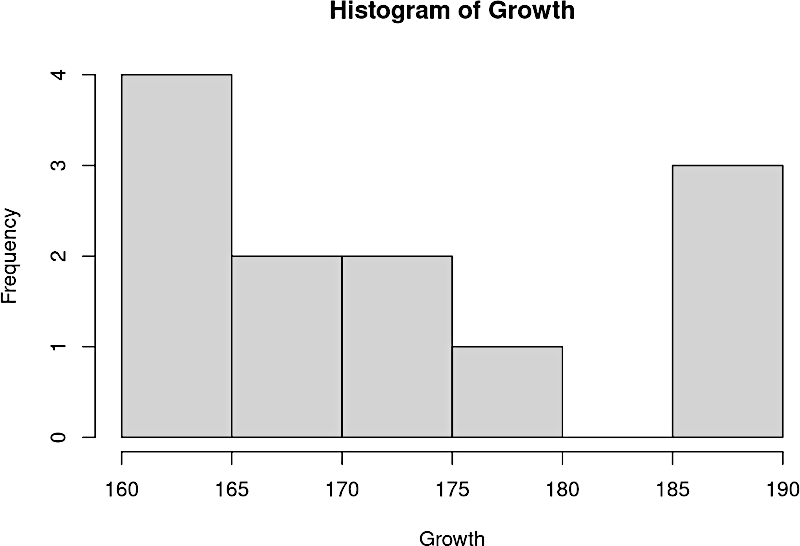

histgrowth


## 
##  Shapiro-Wilk normality test
## 
## data:  Growth
## W = 0.88198, p-value = 0.09292

MSerrorare estimates of between-group and within-group variance, and therefore they can be compared using the F-criterion (Snedecor's criterion, named after Fisher), intended for comparing variances. This criterion is simply the quotient of dividing the larger variance by the smaller one. In our case, it is 420 / 77.2 = 5.440.
Determining the statistical significance of Fisher's criterion using tables
If we were to determine the statistical significance of the effect manually, using tables, we would need to compare the obtained value of the F-criterion with the critical one, which corresponds to a certain level of statistical significance given the degrees of freedom (or "degrees of freedom," as they are called in the source from which the fragment shown in Fig. 11.2.2 is taken).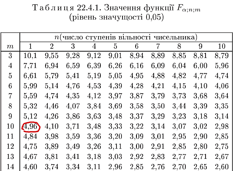

Fig. 11.2.2. A fragment of the table with critical values of the F-criterion (source: Turchyn V.M. Theory of Probability and Mathematical Statistics. Dnipro: IMA-press, 2014. — 556 p.)
As can be seen, for the level of statistical significance p=0.05, the critical value of the F-criterion is 4.96 (as you may remember, dfeffect = 2–1 = 1, and dferror = 12–2 = 10). We obtained a larger value of the criterion; this means that in our example, the effect of the studied sex was registered at the level of statistical significance 0.05.
The obtained result can be interpreted as follows. The probability of the null hypothesis, according to which the mean height of women and men is the same, and the registered difference in their height is due to chance during sample formation, is less than 5%. This means that we should choose the alternative hypothesis, which states that the mean height of women and men in the studied sample differs.
11.3 Analysis in R: The Same or a Different Result?

As you may have noticed, the data we compared using one-way analysis of variance could also be investigated using Student's and Fisher's criteria. Let us compare these two methods. For this, we will calculate the difference in height between men and women using Student's and Fisher's criteria.

We obtained a different result than in the case of one-way analysis of variance. Why? R honestly reported: it used the Welch test. This is related to the fact that the variances of the compared groups are different. This procedure is more correct than the "classical" use of Student's and Fisher's criteria. And how to use the "classical" variant? Tell R that the variances of the compared groups should be considered equal!

	SS	df	MS	F	P
Effect	420,0	1	420,0	5,440	0,041874
5.440	772,0	10	77,2


SampleTest <- aov(Growth~Sex)
summary(SampleTest)


##             Df Sum Sq Mean Sq F value Pr(>F)  
## Sex          1    420   420.0    5.44 0.0419 *
## Residuals   10    772    77.2                 
## ---
## Signif. codes:  0 '***' 0.001 '**' 0.01 '*' 0.05 '.' 0.1 ' ' 1

Як ви могли помітити, ті дані, які ми порівнювали за допомогою однофакторного дисперсійного аналізу, ми могли дослідити і за допомогою критеріїв Стьюдента та Фішера. Порівняємо ці два методи. Для цього обчислимо різницю в зрості чоловіків і жінок з використанням критеріїв Стьюдента і Фішера.


t.test(Growth~Sex)


## 
##  Welch Two Sample t-test
## 
## data:  Growth by Sex
## t = -2.0874, df = 5.454, p-value = 0.08655
## alternative hypothesis: true difference in means between group Female and group Male is not equal to 0
## 95 percent confidence interval:
##  -26.415081   2.415081
## sample estimates:
## mean in group Female   mean in group Male 
##                  168                  180

We obtained a different result than in the case of one-way analysis of variance. Why? R honestly reported: it used Welch's test. This is due to the fact that the variances of the compared groups are different. This procedure is more correct than the "classical" use of the Student's and Fisher's criteria. And how to use the "classical" option? Tell R that the variances of the compared groups should be considered equal!


t.test(Growth~Sex, var.equal = TRUE)


## 
##  Two Sample t-test
## 
## data:  Growth by Sex
## t = -2.3325, df = 10, p-value = 0.04187
## alternative hypothesis: true difference in means between group Female and group Male is not equal to 0
## 95 percent confidence interval:
##  -23.4632431  -0.5367569
## sample estimates:
## mean in group Female   mean in group Male 
##                  168                  180

Now, as we can see, the result is the same as in the case of analysis of variance. It is important to emphasize that although the F-criterion from a mathematical point of view in the analysis by Student's and Fisher's criteria, which we are considering, is the same as in ANOVA (and expresses the ratio of variances), its meaning in the results of the analysis provided by statistical programs is completely different. When comparing by Student's and Fisher's criteria, the comparison of sample mean values is carried out using the Student's criterion, and the comparison of their variability is carried out using the Fisher criterion. The results of the analysis display not the variance itself, but its square root - the standard deviation. On the other hand, in analysis of variance, the Fisher criterion is used to compare the means of different samples (as we discussed, this is done using the distribution of the sum of squares into parts and comparing the mean sum of squares corresponding to between-group and within-group variability). However, the difference noted relates more to the presentation of statistical research results than to its essence. It can be said that comparing groups by Student's criterion can be considered a special case of analysis of variance for two samples. Therefore, comparing samples by Student's and Fisher's criteria has one important advantage over analysis of variance: it allows comparing samples in terms of their variability. But the advantages of analysis of variance are still more significant. These include, for example, the ability to simultaneously compare multiple samples.