Ecology: The Biology of Interactions. VII-02. Introduction to R Properties Through Simple Examples

Appendices: Syllabus. Questions. References. Personalities. Glossary. R Commands.

VII-2. Introduction to R Properties Through Simple Examples
VII-2.1. Using R Markdown
In the previous section (VII-1) we illustrated our discussion by providing screenshots of the RStudio interface. This is an entirely logical approach for an initial introduction to the R working environment, but in general this path is not optimal. In this section we will use the same approach for a time, before transitioning to the use of a more sophisticated tool (also within RStudio). This tool is the R Markdown text markup language, which makes it possible to demonstrate R language commands together with the corresponding output.
R Markdown is a text markup language built into RStudio. It is a means by which RStudio can produce a document that may be converted into many different formats, including .pdf, .html, .docx, and so forth. Its principal advantage is the ability to embed fragments of R scripts and the results of their execution directly within the text.
In general, a fundamental characteristic of scientific writing is its focus not merely on communicating conclusions, but on explaining where those conclusions come from. In the case of simulation modelling and statistical analysis, this means paying particular attention to model parameters, the data being analysed, and the specifics of the algorithms employed. When the subject is a scientific article reporting the results of R-based analysis, one must seek a difficult compromise between the completeness of the text and the ease of its comprehension. It is sometimes necessary to report the principal conclusions in the body of the article while placing the R script with its comments in an appendix. When the text in question is a tutorial, a report, or a qualifying thesis, however, the optimal solution is quite often to combine R code with sufficiently detailed commentary. In cases where the use of hash marks (the # symbol) within the script text is insufficient, R Markdown offers the better solution. Indeed, R Markdown can be useful even for the person who writes an R script or builds an R model themselves. Time passes, and you will forget why you made one choice or another. If you leave a written R Markdown report, you will be able not only to explain your reasoning to someone else; you will make it comprehensible to your future self!
R Markdown documents are created in the same way as R scripts (Fig. VII-2.1). Saved R scripts carry the .R extension, while R Markdown documents carry the .Rmd extension. If you are working under Windows, which conceals important details from the user, you may not have a clear understanding of what an "extension" is; it is the part of a filename that determines the file type and the program that will handle it by default.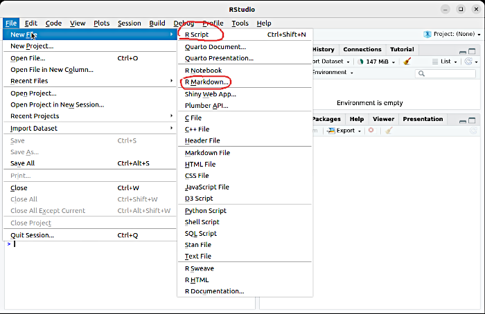

Fig. VII-2.1. An R Markdown document is created in the same way as an R script — through the File menu
R Markdown text may contain special code inserts called chunks. How to create a new chunk is shown in Fig. VII-2.2.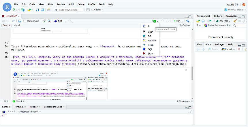

Fig. VII-2.2. Note the two important buttons in an R Markdown document. The green +C button inserts a chunk — a code fragment — while the Knit button depicting a ball of blue yarn converts the document to another format and executes the code within the chunks
As can be seen in Fig. VII-2.2, specific notation is used in R Markdown to convey text formatting elements. At first these notations may seem strange, but they are quite easy to get used to. The main advantage of this language lies in the ability to press the Knit button (literally, "to knit") and obtain a finished document rendered in the desired format. Let us examine the result. In Fig. VII-2.3 you can see a fragment of an R Markdown document containing an R chunk that uses the R function rep(x, times), which creates a vector in which the element x is repeated times times. In this particular case we create a vector vec in which the value 28 is repeated 77 times. We then call (output to the console) the entire vector, and on the next step a single value — the 22nd element. When you read this text in the textbook, you see the result of executing the chunk shown in Fig. VII-2.3. From this point forward we will use precisely this method to demonstrate the results of R execution. To make it possible to reference particular locations in the notes, we will number the chunks (and the R "responses" to them), as is done below.

# Чанк VII-2.1
vec <- rep(28, 77)
vec

##  [1] 28 28 28 28 28 28 28 28 28 28 28 28 28 28 28 28 28 28 28 28 28 28 28 28 28
## [26] 28 28 28 28 28 28 28 28 28 28 28 28 28 28 28 28 28 28 28 28 28 28 28 28 28
## [51] 28 28 28 28 28 28 28 28 28 28 28 28 28 28 28 28 28 28 28 28 28 28 28 28 28
## [76] 28 28

vec[22]

## [1] 28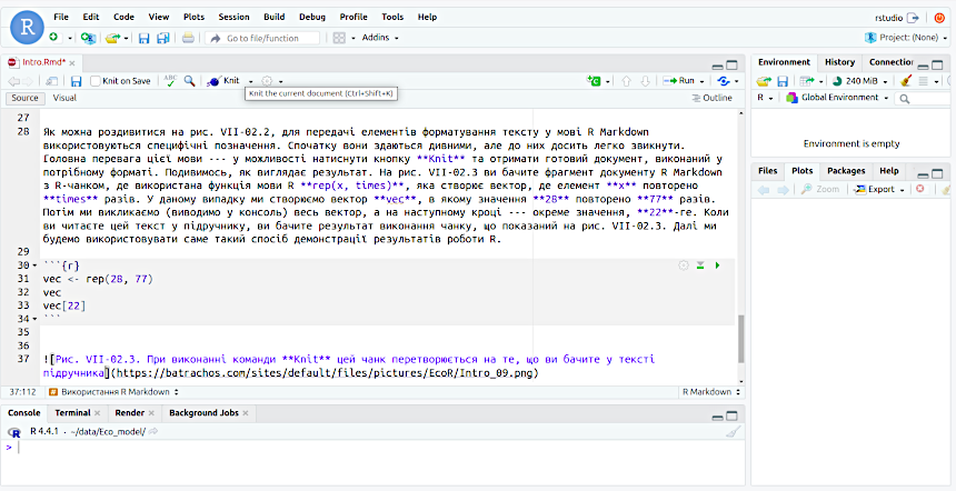

Fig. VII-2.3. When the Knit command is executed, this chunk is transformed into what you see in the body of the textbook VII-2.2. Creating Vectors in R and Their Indexing: Introductory Explanation The basic object type in R is the vector. When we use R, we assign the following meaning to the concept of a "vector" (from the Latin vector — "carrier," "one who carries"): a linear (one-dimensional) sequence of data of a uniform type (for example, numerical data, as in the examples we are about to examine). In other contexts this concept may be used differently; in geometry, for instance, the concept of a vector has an entirely different meaning — it is an object possessing magnitude and direction, that is, a directed line segment. Which definition of this concept is correct? Figure II-1.1 may suggest the appropriate answer. All other objects in R are combinations and modifications of vectors. Even when an R object is a single number, R itself treats it as a vector of unit length. Each element of a vector has its own position, an index within the vector. Accessing individual elements within an object is called indexing. In the chunk shown in Fig. VII-2.3, the following operations occur. vec <- rep(28, 77): the object vec is created, which is a vector containing 77 identical data values. vec: the created vector is directed to the console; in the console output we can see how its elements are indexed: preceding each output line, in square brackets, is the index (number) of the first element in that line. vec[22]: the value of the vector vec at index 22 is output to the console. Note a peculiarity of the R language that distinguishes it from the majority of other programming languages. Indexing within each object begins at 1, not at 0 as in many other languages. Let us examine the command rep(28, 77) more closely. The R function rep() can only be executed if its arguments are specified: what exactly is to be repeated and how many times; this is precisely what the parentheses we included in the function name indicate. Arguments are specified within the parentheses and separated by commas. There are a number of variants for using this command; to become acquainted with them, one may invoke the help associated with the function in question. To do so, one should enter either the command ?rep or the command help(rep) in the script editor or the console; alternatively, one may place the cursor on the relevant word and press F1 on the keyboard. The help commands listed are equivalent; in this example we see that the same result in R can be achieved by different means. Choose from among the approaches described the one that you prefer and use it consistently, or alternatively memorise all of these methods and employ them according to your inclination! Vectors can also be created in various ways. The first five functions in the "Creating objects" section of the appendix listing R commands create precisely vectors. You are already familiar with the : and rep() functions. You can acquaint yourself with the seq() function in its various forms independently (either with the help of the documentation or by experimenting with R, simply offering it different commands and analysing the result). The most important function for creating vectors, c(), requires detailed discussion. The name of the function c() is an abbreviation of combine (some sources indicate a different origin for this name, from the word concatenate, although one might consider that concatenation, "chaining," is performed by other R functions). In any case, the function c() combines the arguments specified within the parentheses and separated by commas into a vector.

# Чанк VII-2.2
v <- c(8, 9, 2, -1, 0.5)

As you know, in different cultures, the decimal separator can be either a dot or a comma. In R, it is always a dot, as in the example provided! In the chunk shown, we created a vector v. It will appear in the Environment window, but upon creation, it will not be displayed in the console. As we indicated, it can be called by a separate command.

# Чанк VII-2.3
v

## [1]  8.0  9.0  2.0 -1.0  0.5

However, objects can be created in such a way that they are immediately sent to the console. To do this, the entire command should be enclosed in parentheses.

# Чанк VII-2.4
(ve <- c(1/3, 2^2, NA, pi))

## [1] 0.3333333 4.0000000        NA 3.1415927

As you know, different cultures use either a period or a comma as the decimal separator. In R it is always a period, as in the example above!
In the chunk above we created the vector v. It will appear in the Environment window, but upon its creation it will not be output to the console. As noted, it can be called with a separate command.

However, objects can be created in such a way that they are immediately directed to the console. To do this, the entire command must be enclosed in parentheses.

What is new in this example? We see that arithmetic expressions (the ^ symbol denotes exponentiation) and certain constants such as the number π can be used in R commands. Note! The element ve[3] is NA, meaning the absence of data, from "not available." If one regards a vector as a linear container for data, one must allow for the possibility that this container may have empty slots.
Incidentally, "multi-level" nested parentheses are quite characteristic of R scripts. RStudio assists in analysing such cases by highlighting the parenthesis that is the counterpart of the one at the current cursor position.
VII-2.3. Elementary Programming: the for() and if() Functions
R is most commonly used for statistical calculations and data analysis. Creating simulation models requires the use of programming constructs to a greater extent than statistical calculations do. The for() and if() functions will be used extensively in the simulation models we will build.
Simulation models often require repeated execution of a given calculation cycle — for example, simulating events occurring within a population each year. Cyclic execution of a given sequence of commands can be organised using the for() loop. Let us create an empty vector and fill it using a loop.

# Чанк VII-2.5
shell <- rep(NA, 10) # Створюємо пустий (заповнений NA) вектор, що буде заповнений даними
length(shell) # Функція length() визначає довжину об'єкта (вектора) 

## [1] 10

shell[1] <- 1 # Задаємо перше значення в векторі shell
for (i in 2:length(shell)) { # В циклі лічильник i перебирає значення в певному векторі
  shell[i] <- shell[i-1] * 2 # Наступне значення розраховується за попереднім
  print(shell[i]) } # Нове значення виводиться на друк у консоль

## [1] 2
## [1] 4
## [1] 8
## [1] 16
## [1] 32
## [1] 64
## [1] 128
## [1] 256
## [1] 512

In the for() loop, the object that will be the loop counter, i.e., the variable that changes its value with each "iteration," should be specified in parentheses. Next, you should specify the vector whose values the counter will sequentially take. In the example given, this is a sequence of integers from 2 to the length of the vector that will change in the loop; this is not mandatory; the sequence of elements in the vector that defines the counter values can be different. Why did we start the loop from value 2? Using the loop, we fill the vector shell. The first, initial value is set manually. All subsequent values, starting from the second, will be calculated using the loop. After the for command, in parentheses, we specify the counter and the vector with its values. Then, after closing the parentheses, we can specify the command to be executed in each "iteration." What if there are several such commands? A series of lines, the commands in which will be executed sequentially under a certain condition, are denoted by curly braces. In the example given, there are two such commands. The first calculates the next value in the vector based on the previous one; for example, when i=2, shell[i] is the second value, and shell[i-1] is the first. The second command, print(), outputs the calculated value to the console. Sometimes a loop needs to be repeated until a certain condition is met. This can usually be achieved in various ways. The first is using a while() loop, the second is using an if() condition inside a for() loop. To get acquainted with the if() condition, let's consider the second option. After the if command, a certain condition is specified in parentheses, and after it – the actions to be performed if this condition is met (of course, this can be a sequential set of commands combined by curly braces). Conditions are expressions that can be true or false; the following operators can be used to construct them: < (less than), > (greater than), <= (less than or equal to), >= (greater than or equal to), == (equal to), != (not equal to). The check for equality may seem unusual; it is not a single equals sign, but two: ==. The fact is that if a single equals sign is used, the first value will be redefined by the second, because in R, not only the assignment operator <- works, but also the operators = and even ->. Why do we use <- specifically? To avoid confusion in different cases; the = operator is mainly used to define function attributes, and alternating <- and -> makes scripts harder for the reader to understand. Let's see how this works using the break command, which terminates the loop execution.

# Чанк VII-2.6
a <- 1
for (a in 1:10000){
  a <- a+1
  if (a==628) break}
a

## [1] 628

The loop "counted up" to the specified value and stopped. The last value of the loop counter, which in this case we designated a, remained in program memory.
VII-2.4. Constructing a Simple Plot Using the plot() Function
The description of R properties presented in this and the preceding section is extremely fragmentary. Its purpose is not a systematic account of the features and capabilities of this modelling tool; attention here has been drawn only to those features that are necessary in order to construct the first model without delay. This will be the subject of the following section.
Before launching the first model, the means for examining the results of modelling are lacking. How can we evaluate what R has produced? We will use the simplest option: a graph.
R is one of the most powerful tools available for scientific graphics. This is attributable above all to specialised packages such as the already-mentioned ggplot2 package. For an initial introduction to R, however, it is better to start with the capabilities built into the base language. We will use the plot() function, since the "philosophy" of its use is simpler. Once you have an example of applying this function to construct, say, a line chart (a diagram demonstrating the dynamics of two variables), you will easily be able to adapt it to your own problems. The plot() function contains a number of arguments that describe the characteristics of the diagram it constructs.
Let us first create two vectors whose dynamics we will represent on the diagram. There is not much intrinsic meaning to these vectors: they are simply an example of two interrelated quantities.

# Чанк VII-2.7
len <- 50 # Максимальна кількість циклів
num <- 10 # Початкові значення в двох векторах
lim <- 1000 # Значення, що зупиняє імітацію
First <- rep(NA, len) # Створення першого вектора
Second <- rep(NA, len) # Створення другого вектора
First[1] <- num # Задаємо перше значення в першому векторі
Second[1] <- num # Те ж саме у другому векторі
for (i in 2:len) { # В циклі лічильник i перебирає значення обмежені величиною len
  First[i] <- First[i-1] + Second[i-1]/5 # Розрахунок наступного значення першого вектора
  Second[i] <- Second[i-1] + First[i-1]/2 # Розрахунок наступного значення другого вектора
  if (max(First[i], Second[i]) > lim) break} # Переривання циклу, якщо значення якогось...
                                                # ... з векторів перевищує значення lim
First[1:i] # Надсилання у консоль заповненої частини першого вектора

##  [1]  10.0000  12.0000  15.0000  19.2000  24.9000  32.5200  42.6300  55.9920
##  [9]  73.6170  96.8412 127.4271 167.6971 220.7098 290.4923 382.3457 503.2484
## [17] 662.3856

Second[1:i] # Надсилання у консоль заповненої частини другого вектора

##  [1]   10.0000   15.0000   21.0000   28.5000   38.1000   50.5500   66.8100
##  [8]   88.1250  116.1210  152.9295  201.3501  265.0636  348.9122  459.2671
## [15]  604.5133  795.6861 1047.3103

In the provided script fragment, three input parameters are set first: len (the number of cycles if the two vectors calculated by the model do not reach the limit value), num (the values from which the dynamics start in both vectors), and lim (the limit value for either of the two vectors that stops the cycle). Then, two empty vectors, First and Second, are created, and their initial values are set according to num. In a loop, the values of these vectors are calculated step by step; the nature of the relationship is chosen arbitrarily (students can experiment with different options by changing the formulas used for recalculation within the loop). At each step, the if() condition checks if the value of either vector has exceeded the planned value lim (the expression max(First[i], Second[i]) selects the larger of the listed values), and if it has, it stops the loop. Finally, the resulting dynamics of both vectors are sent to the console. How to visualize these changes? If we simply pass these two vectors to the plot() function, it will build a diagram at its own discretion.

# Чанк VII-2.8
plot(First, Second)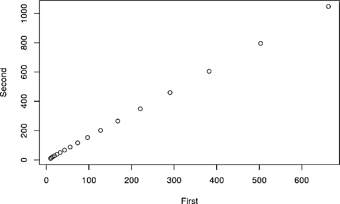

Fig. VII-2.4. The diagram that the plot() function constructs by default when it receives two vectors as input A scatter plot has been constructed, showing for each value of the counter i the corresponding values of the vectors First and Second. How can we compel the plot() function to draw lines showing the values of both vectors as a function of the iteration number? For example, as in the following chunk. Note: the point is not that readers of this text should immediately memorise the commands given. Later, as you build models, you will be able to return to this point to write your own commands by analogy with those given here. On first acquaintance with this fragment it is sufficient to remember that R provides the user with the capabilities listed.

# Чанк VII-2.9
plot(First,  # Побудова найпростішого графіка; джерело даних для першої лінії
     xlim=c(0, i*1.05), # Діапазон значень осі абсцис (осі x)
     ylim=c(0, max(First[i], Second[i])*1.05), # Діапазон значень осі ординат (осі y)
     type="l", # Тип відбиття даних першого вектора (лінія)
     lty=1, # Характер першої лінії (суцільна)
     lwd=1, # Товщина першої лінії (тонка)
     col="blue", # Колір першої лінії
     main="Динаміка двох пов'язаних векторів", # Заголовок графіка
     xlab="Цикли імітації", # Підпис осі абсцис (осі x)
     ylab="Чисельність") # Підпис осі ординат (осі y)
lines(Second, type="l", lty=2, lwd=2, col="red") # Додаємо на графік ще одну лінію
legend("topleft", # Розташування легенди (розшифровки позначень) на графіку
     inset=.05, # Рамка легенди
     title="Вектори", # Назва легенди
     c("перший", "другий"), # Вектор з підписами ліній
     lty=c(1, 2), # Вектор з типами ліній для легенди
     lwd=c(1, 2), # Вектор з товщинами ліній для легенди
     col=c("blue", "red")) # Вектор з кольорами лінії для легенди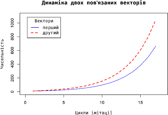

Fig. VII-2.5. This is also the result of the plot() function, but here the user has specified a number of arguments explaining precisely what output is desired The logic here is as follows. First, the plot() function represents the dynamics of the first vector. The xlim= and ylim= arguments define the ranges bounding the coordinate axes. In the example given, the use of the xlim= argument is important in order not to show the "empty" (data-free) portions of the vectors on the diagram; the ylim= argument is provided simply to introduce you to it as well. Note: for these arguments one must specify vectors; in the examples given they are formed by the c() function. Next, in order to represent the dynamics of the vector, one must use the type= argument to specify how the data are represented (points, line, bars, etc., see Fig. VII-2.6); if a line is chosen — the lty= argument defines its type (solid, dashed, see Fig. VII-2.7), and the lwd= argument defines its width (Fig. VII-2.8). The source of these figures is provided here. Three further arguments used specify the chart title and the axis labels. 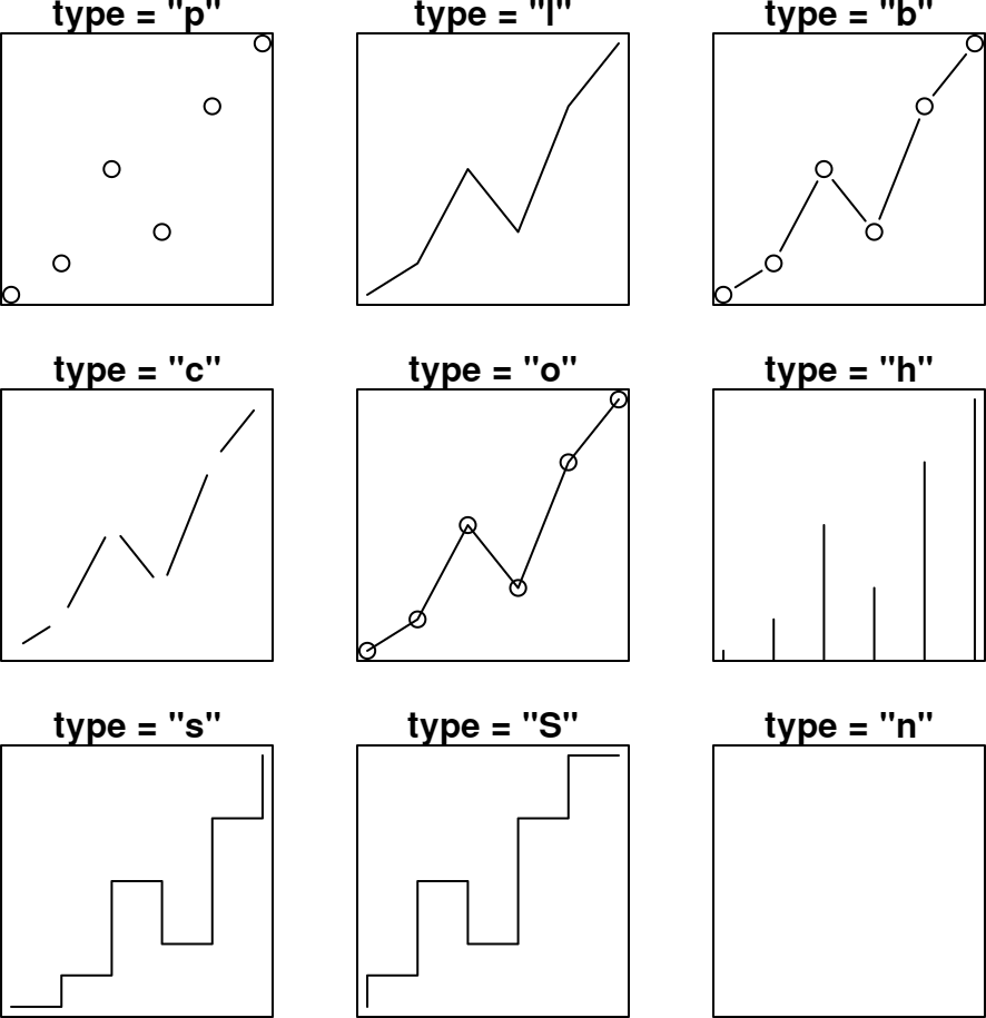Fig. VII-2.6. Types of data representation in the plot() function, specified by the type= argument 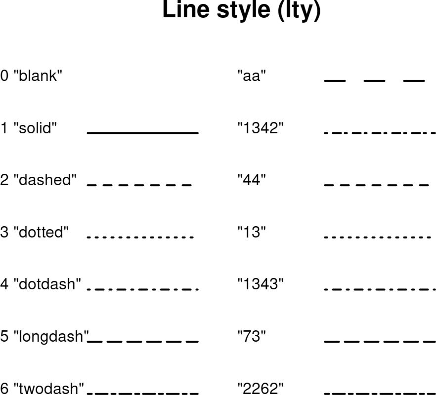Fig. VII-2.7. Line type in the plot() function, specified by the lty= argument 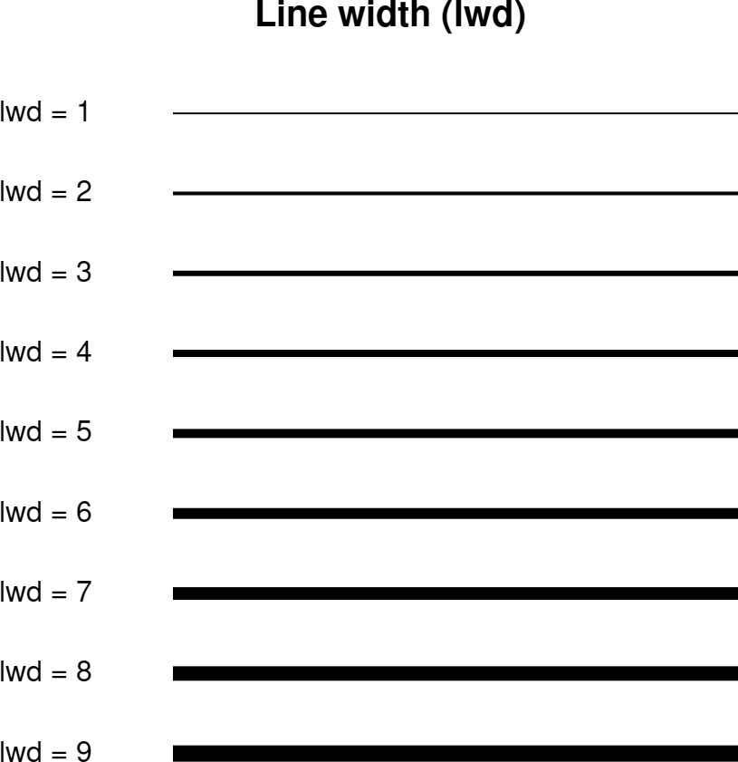Fig. VII-2.8. Line width in the plot() function, specified by the lwd= argument Another characteristic of the line that is specified in the arguments is its colour. There are many ways to specify colour in R; here we will describe the easiest to understand: by name. Colour names are shown in Fig. VII-2.9. 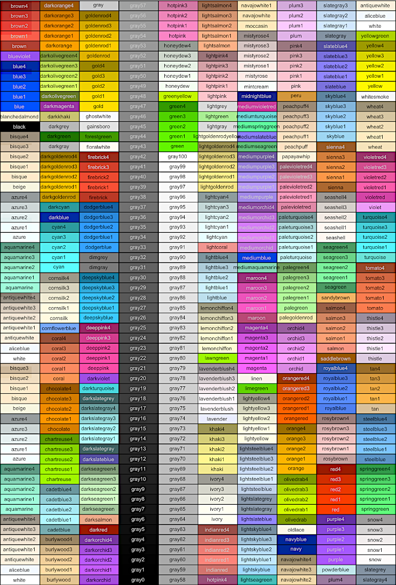Fig. VII-2.9. Colour names in R. If you click on the figure it will open in a full window; on the next click it will be enlarged and easier to examine As you can see, all the arguments we used are specified within the plot() function separated by commas inside the common parentheses (they can all be placed on one line). What happens if these arguments are not specified? Try it! The plot() function will then apply default values. The graph of the first vector has been constructed. How do we add the second vector to it? By adding another line. For this line one must also specify the arguments describing the type of data representation, the line type, and the line width. To make the notation comprehensible, a legend can be added. How can its position on the diagram be specified? By means of such arguments as bottom, bottomleft, left, topleft, top, topright, right, bottomright, center. One can specify the coordinates of the legend. One can choose the option whereby the position of the legend must be specified with the cursor. How? Look it up in the documentation! When specifying the content of the legend, one must again use vectors, listing the characteristics of the symbols and labels that will appear in the legend. Note one further feature reflected in the description of the command supplied as input to the plot() function. It uses not only numerical but also text data — for example, "l", "blue", "Simulation iterations", "topleft", and so forth. Text data are enclosed in quotation marks. RStudio highlights them in green. …Now you are ready to build your first simulation models in R. You are not yet acquainted with the majority of the capabilities and features of this language, but if you have worked through this section and the preceding one, you know what is necessary to construct a simpler model. This is what you will be doing in the next section of this chapter.