
StatOracle–12 Cluster Analysis in R
Cluster analysis — a method very frequently employed in zoological research. Unfortunately, in many instances its application is not the optimal choice, which is precisely why one must understand the distinctive characteristics of this method.
Topic 12 Cluster Analysis in R
(under development)
12.1 Cluster analysis. Is the claim to “objectivity” justified?
Cluster analysis is the general term for a variety of formalised procedures for constructing classifications of objects. Biology was the leading science in the development of cluster analysis. The subject matter of cluster analysis (from the English “cluster” — a bunch, bundle, group) was formulated in 1939 by the psychologist Robert Tryon. The classics of cluster analysis are the American systematists Robert Sokal and Peter Sneath. One of their most important contributions in this field is the book “Principles of Numerical Taxonomy”, published in 1963. In accordance with the central idea of the authors, classification should be constructed not on a compromise between data on similarity and relatedness of objects (sought by insufficiently defined rules), but on the results of formalised processing of mathematically computed similarity/dissimilarity of the classified objects. The procedures appropriate for accomplishing this task were unknown at the time, and the authors therefore set about developing them.
There are two groups of cluster analysis methods — hierarchical (with the construction of a classificatory “tree”, usually represented as a dendrogram) and n-dimensional (with the partitioning of the initial set of objects into a pre-specified number of clusters). In the exposition that follows, we shall primarily consider hierarchical clustering methods.
The main stages of hierarchical cluster analysis are as follows:
1. selection of objects that must be mutually comparable;
2. selection of the set of characters on which the comparison will be based;
3. description of the objects according to these characters;
4. choice of metric — a numerical measure for calculating similarity (or dissimilarity) between objects;
5. calculation of similarity (or dissimilarity) between objects in accordance with the chosen metric;
6. choice of the linkage procedure for grouping objects according to their similarity;
7. the clustering proper: grouping objects into clusters by means of the chosen linkage procedure and recalculating similarities/dissimilarities for the new set of objects until all objects are merged into a single cluster;
8. assessment of the applicability of the obtained cluster solution.
Thus, the most important characteristics of the clustering procedure are the choice of metric (a considerable number of different metrics are used in different situations) and the choice of linkage procedure (here again a considerable number of different options is available for selection). For different situations certain metrics and linkage procedures are more appropriate than others, but to some extent the choice between them is a matter of taste and convention.
The hope that cluster analysis will lead to the construction of a classification entirely independent of the investigator’s arbitrariness (subjective choices) proves unattainable. Of the enumerated stages of a cluster analysis study, the majority — namely stages 1 (choice of objects), 2 (choice of characters), 4 (choice of metric), 6 (choice of linkage procedure), and 8 (decision on the adequacy of the result) — require the adoption of more or less arbitrary decisions that substantially influence the final outcome. This choice may depend on many circumstances, in particular on the explicit and implicit preferences and expectations of the investigator.
Are the described sources of “subjectivity” a fundamental shortcoming specific to cluster analysis? No. For any “objective” methods of analysis these limitations are insurmountable.
Does a single correct solution not exist that determines which objects are more similar and which are less? Let us consider an example.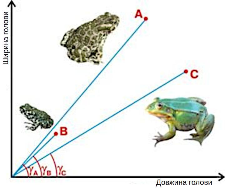
Fig. 12.1.1. Which object is object A more similar to: B or C? If distance is used as the similarity metric, then to C: |AC|<|AB|. But if one relies on characteristic ratios of features? In that case A is more similar to B, since the angle between A and B is smaller than between A and C
So which is correct? In fact, is an adult toad more similar to a juvenile toad or to an adult frog? There is no single correct answer! The answer depends on what is more important to us — the sizes of the objects or their proportions. And what is the “objective” answer? There is no “objectivity” here. If we use, say, scales, the adult specimens are “objectively” similar, while if we focus on species-specific characters, the conspecific individuals are “objectively” similar! The correctness of the answer depends on what we consider more important.
Cluster analysis has found the widest application in modern science. Unfortunately, in a considerable proportion of cases in which it is applied, other methods would have been preferable. In any case, biology specialists must clearly understand the basic logic of cluster analysis, and only then will they be able to apply it precisely in those cases in which it is adequate.
12.2 A worked example of cluster analysis step by step
In order to explain the typical logic of cluster analysis, let us consider a concrete illustrative example. Consider a set of 6 objects (designated by letters), described by 6 characters of the simplest type: alternative characters that take one of two values: present (+) or absent (–). The description of objects by the adopted characters is called the “rectangular” matrix. In our case this is a 6×6 matrix, which may be regarded as entirely “square”, but in general the number of objects in an analysis need not equal the number of characters, and the “rectangular” matrix may have different numbers of rows and columns.
Table 12.2.1. Initial “rectangular” matrix (objects/characters matrix)
| 1 | 2 | 3 | 4 | 5 | 6 | |
| A | – | + | + | – | + | + |
| B | – | + | – | – | – | + |
| C | – | + | – | + | + | – |
| D | + | – | + | – | – | + |
| E | + | – | – | + | – | + |
| F | + | + | – | – | – | + |
Note that the “rectangular” matrix contains the results of the first three stages of cluster analysis that we enumerated in the preceding section. The objects have been selected, the characters have been defined, and the description of the selected objects by the defined characters has been performed.
Next, in order to carry out the cluster analysis, it is necessary to construct a similarity or dissimilarity matrix (the “square” matrix, the objects/objects matrix). For this we must choose a metric — a method for calculating the measure of similarity (dissimilarity) of objects. Since our example has a notional character, it makes sense to choose the simplest possible metric. What is the simplest way to determine the distance between objects A and B when alternative characters are used? By the number of differences between the objects. As can be seen, objects A and B differ with respect to characters 3 and 5, hence the distance between these two objects corresponds to two units. We have completed stage 4 of the study and can proceed to stage 5. Using the chosen metric, we construct the “square” matrix (the objects/objects matrix). As can easily be verified, such a matrix consists of two symmetrical halves, and only one of them needs to be filled in.
Table 12.2.2. Initial “square” matrix (objects/objects matrix)
| A | B | C | D | E | F | |
| A | — | 2 | 3 | 3 | 5 | 3 |
| B | — | 3 | 3 | 3 | 1 | |
| C | — | 6 | 4 | 4 | ||
| D | — | 2 | 2 | |||
| E | — | 2 | ||||
| F | — |
In this case we have constructed a dissimilarity matrix. A similarity matrix would have a similar appearance, except that at each position would stand a value equal to the difference between the maximum distance (6 units) and the dissimilarity between the objects. Thus for the pair A and B the similarity would be 4 units.
Before proceeding to the clustering procedure, we must choose the linkage method for joining an object to a cluster. As a rule, when we are dealing with a set of individual objects as in the matrix above, no particular difficulties arise. In the matrix above, the closest pair of objects is B and F, which differ in only one character. The essence of cluster analysis lies in joining similar objects into a cluster. After such joining a new object arises — the cluster (BF). Parentheses in our notation denote the merging of formerly separate units into a single whole. After two former objects have been eliminated and a new one formed, the corresponding segments of the “square” matrix will need to be recalculated.
Object A is at a distance of 2 units from object B, and 3 units from F. What is the distance from A to (BF)?
Perhaps the distance from an object to a group is the distance from the object to the nearest object within the group, i.e., |A(BF)|=|AB|? This logic corresponds to the single linkage (nearest-neighbour) method. In that case the distance we compute is 2 units.
Alternatively, the distance from an object to a group might be the distance from the object to the farthest object within the group, i.e., |A(BF)|=|AF|? This logic corresponds to the complete linkage (farthest-neighbour) method, yielding a distance of 3 units.
One may also consider the distance from an object to a group to be the arithmetic mean of distances from that object to each of the objects within the group, i.e., |A(BF)|=(|AB|+|AF|)/2. This solution is termed average linkage. The distance in that case is 2.5 units.
The examples given do not exhaust the diversity of linkage methods. For instance, Ward’s method compares by how much each possible decision about merging objects increases the total within-cluster variance; other variants are also possible. And how should objects be joined “objectively”? It depends on what is more important to us, and on what shape and internal diversity we wish the clusters to have. For example, single linkage ultimately produces long, “chain-like” clusters, while complete linkage tends to produce compact, spherical clusters. Once again — “damned indeterminacy”!
Suppose we have chosen the simplest linkage method — average linkage (UPGMA). In that case we can proceed to repeating stage 7 of the algorithm we have described. The first step of this process we have already described: merging B and F into (BF). Let us illustrate this on a diagram. As can be seen, the objects are joined at the level corresponding to the distance between them.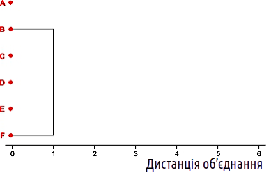
Fig. 12.2.1. First step of clustering
Now we have not six objects but five. We reconstruct the “square” matrix taking into account the chosen linkage method.
Table 12.2.3. “Square” matrix after the first step of clustering (5×5)
| A | (BF) | C | D | E | |
| A | — | 2,5 | 3 | 3 | 5 |
| (BF) | — | 3,5 | 2,5 | 2,5 | |
| C | — | 6 | 4 | ||
| D | — | 2 | |||
| E | — |
Now the closest pair of objects is D and E. Let us merge them as well.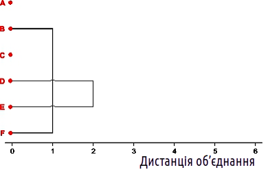
Fig. 12.2.2. Second step of clustering
Table 12.2.4. “Square” matrix after the second step of clustering (4×4)
| A | (BF) | C | (DE) | |
| A | — | 2,5 | 3 | 4 |
| (BF) | — | 3,5 | 2,5 | |
| C | — | 5 | ||
| (DE) | — |
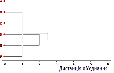
After the second step we see that there are two possible mergers at the level of 2.5: joining A to (BF) and joining (BF) to (DE). Which should be chosen?
We have various options for making such a choice. It can be made randomly. A formal rule may be adopted that permits a choice to be made. Or one can examine which of the decisions yields the best clustering result. Let us follow the last path: we shall calculate both variants and see which produces the better result.
|
—
|
After the second step we see that there are two possible mergers at the level of 2.5: joining A to (BF) and joining (BF) to (DE). Which should be chosen?
|
||||||||||||||||||||||||||||||||
|
We have various options for making such a choice. It can be made randomly. A formal rule may be adopted that permits a choice to be made. Or one can examine which of the decisions yields the best clustering result. Let us follow the last path: we shall calculate both variants and see which produces the better result. A. |
|||||||||||||||||||||||||||||||||
A.
|
B.
|
||||||||||||||||||||||||||||||||
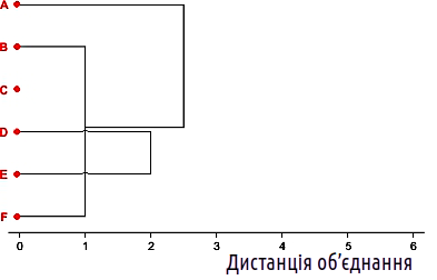
A.
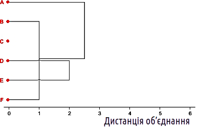
| (AC) | (BFDE) | |
| (AC) | — | 3,625 |
| (BFDE) | — |
B. 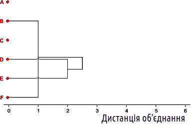
Fig. 12.2.3. Alternative variants for the third step of clustering
Table 12.2.5. Two variants of “square” matrices after the third step of clustering (3×3)
B.
The resulting 3×3 matrices (Table 12.2.5) can be compared, and one can verify that a more compact grouping of objects is achieved in variant B. When constructing a classification of objects by means of cluster analysis, we should strive to identify groups that unite similar objects. The greater the within-group similarity of objects, the better such a classification. Therefore for the third step of clustering we choose variant B.
In that case, the next step is to merge objects A and C.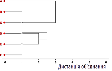
Fig. 12.2.4. Fourth step of clustering
Table 12.2.6. “Square” matrix after the fourth step of clustering (2×2)
Now there is no choice to be made. We merge the two remaining clusters at the required level. In accordance with the accepted convention for constructing cluster “trees”, we add a “trunk” extending to the level of the maximum possible distance between objects given this character set.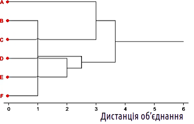
Fig. 12.2.5. The fifth and final step of clustering; however, such a tree does not look its best
The resulting picture is a tree-like graph (a set of vertices and connections between them). This graph is constructed such that the lines forming it cross one another (we have indicated these crossings with “bridges”). Without changing the connectivity between objects the graph can be redrawn so that it contains no crossings whatsoever. The point is that such a graph can shift its branches without loss of topology, much as a spider can rearrange its legs. The final result is shown in Fig. 12.2.6.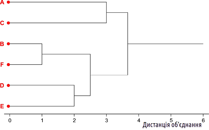
Fig. 12.2.6. The final clustering result. The resulting tree looks attractive, but, looking at it, try to find the answer: which object is object A closer to: B or F?
How should the graph shown in Fig. 12.2.6 be interpreted? There is no unambiguous answer. On the surface lies the conclusion that we have registered the initial set of 6 objects as consisting of three pairs. Looking at the obtained plot, it is hard to doubt this. However, is this conclusion entirely correct?
Return to the very first “square” 6×6 matrix (Table 12.2.2) and verify: object E was at a distance of two units from both object D and object F. The similarity of E and D is reflected in the final “tree”, but the fact that object E was equally close to object F has been lost without trace! How can this be explained? In the clustering result shown in Fig. 12.2.6, information about the distance |EF| is entirely absent; only information about distances |DE| and |(BF)(DE)| is present! An analogous situation exists with the question posed in Fig. 12.2.6. The necessary information is contained in Table 12.2.2 and in the descriptions of the objects (Table 12.2.1). But at the stage reflected in the final figure, this information is no longer present (you will recall that the “spider legs” of the graph can be rearranged in any way).
Each “rectangular” matrix, given a particular choice of metric and linkage method, corresponds to one and only one “square” matrix. However, each “square” matrix may correspond to many “rectangular” matrices. After each step of the analysis each preceding “square” matrix corresponds to the subsequent one, but from the subsequent matrix we could not recover the preceding one. This means that at each step of cluster analysis a certain portion of information about the diversity of the initial set of objects is irreversibly lost.
12.3 “Methodological” conclusions
Could it be that the irreversible information loss at each step of clustering represents a fundamental shortcoming of cluster analysis, from which other methods are free? No. The task of classification and ordination methods is to reduce the quantity of information pertaining to the comparison of objects. This is precisely the strength of cluster analysis: instead of the enormous unstructured information reflecting the pairwise comparison of objects, we obtain the most characteristic portion of this information embodied in the constructed tree. Which portion of the data on similarities and dissimilarities of objects is most important to us is determined by the decisions we have made regarding the choice of metric and linkage method.
A certain shortcoming of cluster analysis in comparison with other classification and ordination methods is that the information loss we have described is relatively concealed. Principal components analysis reports what proportion of the initial information is reflected by each component; non-metric multidimensional scaling outputs stress information. When it comes to cluster analysis, however, users with insufficient experience do not notice such information loss — which is precisely why we have expended such effort to demonstrate it.
Of course, the fairy-tale hope for “objectivity” is unattainable. Cognition — that is, the construction by a particular subject of a model of some aspect of reality — is subjective by definition. Depending on which initial data are taken for model construction and toward which goal this model is built, entirely different results may be obtained. This need not be combated; it must be accepted as a given. But does concern for “objectivity” have at least some meaning?
It does. Often when the antinomy “objectivity – subjectivity” is invoked, what is actually meant is something different: “unbiasedness – bias”. If cluster analysis (and any other method) becomes a means of obtaining a predetermined result (and if the initial data do not conform to this result — so much the worse for the initial data!), statistical analysis becomes a tool of manipulation and deception. We must not proceed toward a predetermined destination, but must move in the direction to which the empirical data lead us.
So when does hierarchical cluster analysis make sense to use? When there are grounds to expect that the structure of similarities and dissimilarities of the classified objects reflects a certain hierarchy. When might this occur? We provide examples.
— the similarities and differences among species, being consequences of their evolution, reflect the sequence of branching events in the evolutionary tree uniting them;
— the diversity of samples reflects the action of factors of different weights; for example, the composition of benthic samples depends more strongly on the type of water body and less so on depth;
— the cells in a blood sample differ primarily by their histological type and secondarily by individual characteristics.
When there are no grounds to expect that the diversity of the classified objects is organised hierarchically, the use of cluster analysis is unjustified. If in the multidimensional space the objects form tight groups that are themselves components of larger groups and so on, cluster analysis will find and display this structure. But what will happen if the mutual arrangement of objects does not reflect a hierarchy of smaller or larger groups? In that case cluster analysis will create such a hierarchy artificially, because that is precisely how its algorithms work.
Imagine a typical situation. An investigator analyses the similarities and dissimilarities of objects distributed randomly (or, say, normally) in multidimensional space. The investigator applies hierarchical cluster analysis and… obtains a certain hierarchy reflected in the dendrogram that this analysis constructs. And the investigator accepts this as proof that such a hierarchy exists in the initial data! In such a case it is useful to reflect on the following question — is it possible not to obtain a hierarchical structure using a method whose sole capability is to construct a hierarchical structure?
Why, then, is hierarchical cluster analysis so popular? It constructs a structure that appears simple to perceive — a tree. It became widespread in an era when the investigator’s capabilities were severely constrained by computational limitations (one of the authors of this textbook published in the previous century a paper in which cluster analysis was performed “by hand”, as in the example given in the preceding section). Even experienced investigators are primates and therefore imitate the analytical tools used by other primates…
What should be done then? Use cluster analysis only when it makes sense — when there are grounds to expect that the mutual arrangement of the classified objects reflects a certain hierarchy of factors generating diversity. Incidentally, when such a hierarchy exists, different metrics and different linkage methods will yield comparable and relatively coherent results; in the absence of such a hierarchy, the result will be unstable. And if there are no grounds for using cluster analysis, it is better to employ ordination methods — principal components analysis, non-metric multidimensional scaling, and so forth.
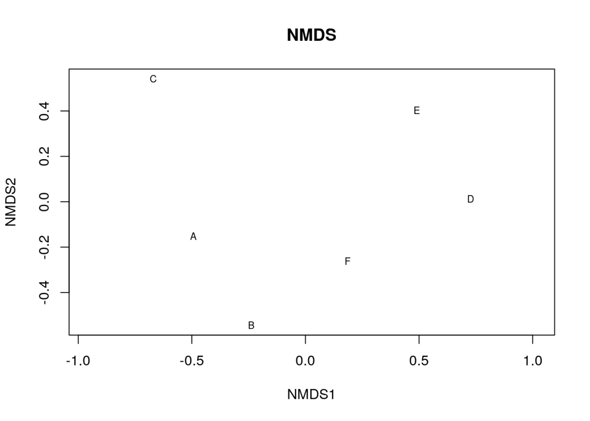
Although non-metric multidimensional scaling will be covered in the next chapter, we present here the result of performing this analysis on the same dataset that was used for the clustering.
| 1 | 2 | 3 | 4 | 5 | 6 | |
| A | – | + | + | – | + | + |
| B | – | + | – | – | – | + |
| C | – | + | – | + | + | – |
| D | + | – | + | – | – | + |
| E | + | – | – | + | – | + |
| F | + | + | – | – | – | + |
Note that the "rectangular" matrix contains the results of the first three stages of cluster analysis, which we listed in the previous point. Objects are selected, features are defined, and the description of selected objects by defined features has been carried out. Next, to perform cluster analysis, it is necessary to construct a similarity or difference matrix (a "square" matrix, an objects/objects matrix). To do this, we need to choose a metric - a way to calculate the measure of similarity (or difference) between objects. Since our example is conditional, it makes sense to choose the simplest metric. How to most simply determine the distance between objects A and B, under conditions where alternative features are used? By the number of differences between objects. As you can see, objects A and B differ in features 3 and 5, a total of two differences, i.e., the distance between these two objects corresponds to two units. We have completed the 4th stage of the research and can move on to the 5th. Using the chosen metric, let's construct a "square" matrix (objects/objects matrix). As can be easily verified, such a matrix consists of two symmetrical halves, and only one of them can be filled. Table 12.2.2. Initial "square" matrix (objects/objects matrix)
| A | B | C | D | E | F | |
| A | — | 2 | 3 | 3 | 5 | 3 |
| B | — | 3 | 3 | 3 | 1 | |
| C | — | 6 | 4 | 4 | ||
| D | — | 2 | 2 | |||
| E | — | 2 | ||||
| F | — |
In this case, we have constructed a difference matrix. A similarity matrix would have a similar appearance, only at each position there would be a value equal to the difference between the maximum distance (6 units) and the difference between the objects. Thus, for the pair A and B, the similarity would be 4 units. Before moving on to the clustering procedure, we should choose a method for attaching an object to a cluster. Usually, when we deal with a set of individual objects, as in the given matrix, there are no particular issues. In the given matrix, objects B and F are closest, differing by only one feature. The essence of cluster analysis is to combine similar objects into a cluster. After such a combination, a new object is formed - a cluster (BF). Parentheses in this case in our notation denote the combination of former individual units into a single whole. After two former objects disappear and a new one is formed, the corresponding fragments of the "square" matrix will need to be recalculated. Object A is at a distance of 2 units from object B, and 3 from F. What is the distance from A to (BF)? Perhaps the distance from an object to a group is the distance from the object to the closest object in the group, i.e., |A(BF)|=|AB|? This logic corresponds to attachment by maximum similarity. In this case, the distance we calculate is 2 units. Or perhaps the distance from an object to a group is the distance from the object to the farthest object in the group, i.e., |A(BF)|=|AF|? This logic corresponds to attachment by minimum similarity, the distance is 3 units. It is also possible to consider that the distance from an object to a group is the arithmetic mean of the distances from this object to each of the objects in the group, i.e., |A(BF)|=(|AB|+|AF|)/2. This solution is called attachment by average similarity. The distance in this case is 2.5 units. The examples given do not exhaust the variety of attachment methods. For example, Ward's method compares how much each possible decision to combine objects increases the total variance within objects; other options are also possible... And how should objects be combined "objectively"? Depending on what is more important to us, what kind of clusters, in terms of shape and internal diversity, we will build. For example, attachment by maximum similarity ultimately leads to the formation of long, "ribbon-like" clusters. By minimum similarity - to the fragmentation of groups. Again, "damned uncertainty"! Let's assume we chose the simplest method of combination - by average similarity. In this case, we can proceed to repeat the 7th stage of the algorithm described by us. We have already described the first step of such a process: combining B and F into (BF). Let's show this on a diagram. As you can see, the objects are combined at the level corresponding to the distance between them. Fig. 12.2.1. First step of clustering Now we have not six objects, but five. We rebuild the "square" matrix taking into account the chosen combination method. Table 12.2.3. "Square" matrix after the first step of clustering (5x5)
| A | (BF) | C | D | E | |
| A | — | 2,5 | 3 | 3 | 5 |
| (BF) | — | 3,5 | 2,5 | 2,5 | |
| C | — | 6 | 4 | ||
| D | — | 2 | |||
| E | — |
Now the closest pair of objects is D and E. Let's combine them too. Fig. 12.2.2. Second step of clustering Table 12.2.4. "Square" matrix after the second step of clustering (4x4)
| A | (BF) | C | (DE) | |
| A | — | 2,5 | 3 | 4 |
| (BF) | — | 3,5 | 2,5 | |
| C | — | 5 | ||
| (DE) | — |
After the second step, we see that there are two possibilities for the next combination at the level of 2.5: attaching A to (BF) and attaching (BF) to (DE). Which one to choose? We have various options for making such a choice. It can be made randomly. A formal rule can be adopted that allows making a choice. Or we can see which of the options gives the best clustering result. Let's go the latter way: we will calculate both options and see which one gives a better result.
|
— |
After the second step we see that there are two possible mergers at the level of 2.5: joining A to (BF) and joining (BF) to (DE). Which should be chosen?
|
||||||||||||||||||||||||||||||||
|
We have various options for making such a choice. It can be made randomly. A formal rule may be adopted that permits a choice to be made. Or one can examine which of the decisions yields the best clustering result. Let us follow the last path: we shall calculate both variants and see which produces the better result. A. |
|||||||||||||||||||||||||||||||||
A.
|
B.
|
||||||||||||||||||||||||||||||||
The obtained 3x3 matrices (Table 12.2.5) can be compared, and it can be confirmed that a more compact grouping of objects is achieved in variant B. When constructing a classification of objects using cluster analysis, we should strive to identify groups that combine similar objects. The higher the similarity of objects within groups, the better such a classification. Therefore, for the third step of clustering, we choose variant B. In this case, the next step is to combine objects A and C. Fig. 12.2.4. Fourth step of clustering Table 12.2.6. "Square" matrix after the fourth step of clustering (2x2)
| (AC) | (BFDE) | |
| (AC) | — | 3,625 |
| (BFDE) | — |
Now there is nothing to choose from. We combine the two remaining clusters at the required level. According to the accepted style of constructing cluster "trees", we will add a "trunk" that extends to the level of the maximum possible distance between objects for the given set of features. Fig. 12.2.5. Fifth, final step of clustering; however, such a tree does not look the best. The resulting picture is a tree-like graph (a set of vertices and connections between them). This graph is constructed in such a way that the lines forming it intersect (we have shown these intersections with "bridges"). Without changing the nature of the connections between objects, the graph can be rebuilt so that there are no intersections. The point is that such a graph can move its branches without losing its topology, just as a spider can move its legs. The final result is shown in Fig. 12.2.6. Fig. 12.2.6. Final clustering result. The resulting tree looks attractive, but looking at it, try to find the answer: to which object is object A closer: to B or to F? How to interpret the graph shown in Fig. 12.2.6? There is no unambiguous answer. The conclusion that we registered that the initial set of 6 objects consists of three pairs lies "on the surface." Looking at the resulting graph, it is hard to doubt this. However, is this conclusion entirely valid? Go back to the very first "square" matrix 6x6 (Table 12.2.2) and make sure: object E was at a distance of two units from both object D and object F. The similarity of E and D is reflected in the final "tree", but the fact that object E was as close to object F is lost without a trace! How to explain this? In the clustering result shown in Fig. 12.2.6, there is no information about the distance |EF|, only information about the distances |DE| and |(BF)(DE)|! The situation is analogous to the question posed in Fig. 12.2.6. The necessary information is contained in Table 12.2.2 and in the object descriptions (Table 12.2.1). And at the stage reflected in the last figure, this information is missing (you remember that the "spider legs" of the graph can be moved as you like?). Each "rectangular" matrix, in the case where a certain metric and combination method are chosen, corresponds to a single "square" matrix. However, many "rectangular" matrices can correspond to one "square" matrix. After each step of the analysis, each previous "square" matrix corresponds to the next one, but, based on the next one, we could not restore the previous one. This means that at each step of cluster analysis, a certain part of the information about the diversity of the initial set of objects is irreversibly lost. 12.3 "Methodological" conclusions Perhaps the fact that at each step of clustering, part of the information about the similarities and differences of objects is lost, hides a fundamental flaw of cluster analysis, and other methods are free from similar flaws? No. The task of classification and ordination methods is to reduce the amount of information related to the comparison of objects. This is the strength of cluster analysis: instead of a huge amount of unstructured information reflecting the comparison of objects, we get an embodiment of the most characteristic part of this information in the constructed tree. Which part of the information about the similarities and differences of objects is most important to us is determined by the decisions we make regarding the choice of metric and combination method. A certain drawback of cluster analysis compared to other classification and ordination methods is that the information loss described by us is relatively hidden. The principal component method reports what part of the initial information is reflected in each component; non-metric scaling shows stress information. But when it comes to cluster analysis, insufficiently experienced users do not notice such information loss - that is why we spent so much effort to demonstrate it. Of course, the fairy-tale hope for "objectivity" is unattainable. Cognition - that is, the construction by a certain subject of a model of some aspect of reality - is subjective by definition. Depending on what initial data are taken for the construction of the model, for what purpose this model is built, completely different results can be obtained. This should not be fought; it should be accepted as a given. But does concern for "objectivity" make any sense at all? It does. Often, when they talk about the antinomy of "objectivity - subjectivity", they actually mean something else: "impartiality - bias". If cluster analysis (and any other method) becomes a way of obtaining a predetermined result (and if the initial data do not correspond to this result - so much the worse for the initial data!), then statistical analysis becomes a way of manipulation, deception. We should not go to a predetermined point, but we should move where the empirical data lead us. So when does it make sense to use hierarchical cluster analysis? When there are reasons to expect that the structure of similarities and differences of classified objects reflects a certain hierarchy. When can this happen? Let's give examples. - similarities and differences of species, resulting from their evolution, reflect the sequence of branching of the evolutionary tree that connects them; - the diversity of samples reflects the action of factors of different weights, for example, the composition of benthic samples depends more on the type of water body, and less significantly - on depth; - cells in a blood sample differ primarily by their histological type, and secondarily by individual characteristics. When there are no reasons to expect that the diversity of classified objects is organized hierarchically, the use of cluster analysis is unjustified. If in a multidimensional space objects form tight groups that are part of larger groups, and so on, cluster analysis will find and demonstrate this structure. What happens if the relative position of objects does not reflect a certain hierarchy of smaller or larger groups? In this case, cluster analysis will create such a hierarchy artificially, because that is how its algorithms work. Imagine a typical situation. A researcher analyzes the differences and similarities of objects randomly (or, let's assume, normally) located in multidimensional space. They apply hierarchical cluster analysis and... obtain a certain hierarchy, reflected in the dendrogram that this analysis builds. And the researcher takes this as proof that such a hierarchy exists in the initial data! In this case, it is useful to consider the question - is it possible not to obtain a hierarchical structure using a method that can only build a hierarchical structure? And why is hierarchical cluster analysis so popular? It builds a structure that seems simple to perceive - a tree. It spread in times when researchers' capabilities were very limited by computational power (one of the authors of this textbook published a paper in the last century where cluster analysis was performed "manually", as in the example given in the previous section). Even experienced researchers are monkeys and therefore mimic the analysis tools used by other monkeys... What should be done? Use cluster analysis only when it makes sense, if there are reasons to expect that the relative positions of classified objects reflect a certain hierarchy of factors generating diversity. By the way, if such a hierarchy exists, different metrics and different methods of combining clusters will give comparable and relatively understandable results; if it does not exist, the result will be unstable. And if there are no grounds to use cluster analysis, it is better to use ordination methods - principal component analysis, non-metric scaling, etc. Although non-metric scaling will be discussed in the next section, we will provide the result of performing this analysis for the dataset for which we did clustering here.
library(vegan)
A <- c(0, 1, 1, 0, 1, 1)
B <- c(0, 1, 0, 0, 0, 1)
C <- c(0, 1, 0, 1, 1, 0)
D <- c(1, 0, 1, 0, 0, 1)
E <- c(1, 0, 0, 1, 0, 1)
F <- c(1, 1, 0, 0, 0, 1)
NmSc <- data.frame(A, B, C, D, E, F)
NmSc_t <- t(NmSc)
dist_matrix <- vegdist(NmSc_t, method = "jaccard", binary = TRUE)
nmds_result <- metaMDS(dist_matrix, k = 2, trymax = 100)
nmds_result
##
## Call:
## metaMDS(comm = dist_matrix, k = 2, trymax = 100)
##
## global Multidimensional Scaling using monoMDS
##
## Data:     dist_matrix
## Distance: binary jaccard
##
## Dimensions: 2
## Stress:     0.02844537
## Stress type 1, weak ties
## Best solution was repeated 3 times in 20 tries
## The best solution was from try 0 (metric scaling or null solution)
## Scaling: centring, PC rotation, halfchange scaling
## Species: scores missing
plot(nmds_result, type = "t", main = "NMDS")