Ecology: the biology of interaction. VII-06. Approximation of data on global human population growth using various models

VII-6. Approximation of Global Human Population Growth Data Using Various Models
What mathematical relationship best describes the growth in the number of representatives of our species on Earth? For this purpose, we can use estimates of human population size at various stages of its history. Of course, these estimates are not absolutely accurate, but they are the best we have, and based on them, we can draw many conclusions. Let's start by creating vectors for time markers and human population size.
These data are also provided in the corresponding section of the textbook, but the simplest way to obtain them while working with R is to simply copy the commands provided here.


t <-c(-10000, -5000, -4000, -3000, -2000, -1000, -500, -200, 0, 200, 600, 700, 800, 900, 1000, 1100, 1400, 1200, 1500, 1650, 1700, 1760, 1804, 1850, 1900, 1927, 1950, 1951, 1952, 1953, 1954, 1955, 1956, 1957, 1958, 1959, 1960, 1961, 1962, 1963, 1964, 1965, 1966, 1967, 1968, 1969, 1970, 1971, 1972, 1973, 1974, 1975, 1976, 1977, 1978, 1979, 1980, 1981, 1982, 1983, 1984, 1985, 1986, 1987, 1988, 1989, 1990, 1991, 1992, 1993, 1994, 1995, 1996, 1997, 1998, 1999, 2000, 2001, 2002, 2003, 2004, 2005, 2006, 2007, 2008, 2009, 2010, 2011, 2012, 2013, 2014, 2015, 2016, 2017, 2018, 2019, 2020, 2021, 2022, 2023, 2024, 2025, 2026)
N <-c(4000000, 5000000, 7000000, 14000000, 27000000, 50000000, 100000000, 150000000, 170000000, 190000000, 200000000, 210000000, 220000000, 240000000, 275000000, 320000000, 350000000, 360000000, 450000000, 500000000, 610000000, 770000000, 1000000000, 1200000000, 1600000000, 2000000000, 2493092848, 2536927035, 2584086339, 2634106235, 2685894860, 2740213792, 2795409994, 2852618337, 2911249671, 2965950351, 3015470894, 3064869675, 3123374315, 3192807828, 3264487339, 3334533703, 3404041125, 3473412880, 3545187251, 3619491579, 3694683794, 3769847865, 3844917680, 3920805042, 3996416096, 4070735277, 4144246377, 4217863796, 4292097502, 4368539528, 4447606236, 4528777306, 4612673421, 4697327573, 4782175519, 4868943465, 4958072838, 5049746397, 5141992542, 5234431732, 5327803110, 5418735891, 5505989816, 5591544797, 5675551255, 5758878982, 5842055734, 5924787816, 6007066690, 6089006339, 6171702993, 6254936459, 6337730342, 6420361634, 6503377772, 6586970132, 6671452015, 6757308781, 6844457662, 6932766416, 7021732148, 7110923765, 7201202485, 7291793585, 7381616244, 7470491872, 7558554526, 7645617954, 7729902781, 7811293698, 7887001292, 7954448391, 8021407192, 8091734930, 8161972572, 8231613070, 8300678395)

We will use models for approximating the data presented that can only be applied with a large error. The sums of squared residuals will be relatively large. To work with numbers of a smaller scale, it is convenient to use population data in millions of people. For this, it is sufficient to divide the values in vector N by a million to obtain vector N_mil. The scientific notation format is used in the command below; it should be remembered that 1000000 = 1e6 = 1×exp(6) = 1×e6.


N_mil <- N / 1e6

If we needed a data matrix, we could create it from vectors in a very simple way – for example, as shown below. However, there is no need for this; we will work with two vectors.


WorldPop <- cbind(t, N_mil)
tail(WorldPop)


##           t    N_mil
##  [98,] 2021 7954.448
##  [99,] 2022 8021.407
## [100,] 2023 8091.735
## [101,] 2024 8161.973
## [102,] 2025 8231.613
## [103,] 2026 8300.678

Let's start with the simplest (and obviously not very effective) method of data approximation, we will use a simple linear relationship. As is known, a straight line is defined by the formula N = a t + b, where a is the slope of the line, and b is its intercept. In our case, it is better to use the formula N t = (t - t 0 ) a + N 0. The parameter b is determined by the ratio of t 0 and N 0. We will use the lm() function, which is used to calculate linear regression. The arguments in parentheses for this function mean "the dependence of N_mil on t". We obtain the dependence, save it under the name fit_lin, and extract the required parameters from it.


fit_lin <- lm(N_mil ~ t)
a_val <- coef(fit_lin)[2]
intercept <- coef(fit_lin)[1]
t0_fixed <- -10000 
N0_val <- intercept + a_val * abs(t0_fixed)

To measure the model's fit to the data on which it is built, RSS (Residual sum of squares) is used. Let's calculate it to be able to compare the linear model with those that will be created later.


rss_lin <- deviance(fit_lin)

The next step is exponential growth. N t = N 0 * exp(r * (t - t 0_fixed )). If we logarithmize the exponential dependence, we get a straight line, and thus, this problem can be reduced to the previous one. However, we will use the optimization procedure to fit the parameters specifically in the exponential model. Initial parameter values can be obtained using the lm() command applied to the log-transformed data: log(N) = log(N 0 ) + r × (t - t 0_fixed ).


log_fit <- lm(log(N_mil) ~ I(t - t0_fixed))
start_N0 <- exp(coef(log_fit)[1])
start_r <- coef(log_fit)[2]

We will use the obtained data as a starting point for optimizing the parameters of the exponential equation. The task is not simple (the available data differ greatly from exponential growth), but we will use a relatively stable "port" algorithm and, using the minFactor settings, allow very minor improvements during optimization.


fit_exp <- nls(N_mil ~ N0 * exp(r * (t - t0_fixed)), 
               start = list(N0 = start_N0, r = start_r),
               algorithm = "port",
               control = nls.control(maxiter = 1000, 
                                     minFactor = 1/4096, 
                                     warnOnly = TRUE))


## Warning in nls(N_mil ~ N0 * exp(r * (t - t0_fixed)), start = list(N0 =
## start_N0, : Convergence failure: function evaluation limit reached without
## convergence (9)


params_exp <- coef(fit_exp)
N0_res <- params_exp["N0"]
r_res <- params_exp["r"]

Let's calculate the RSS for the exponential model.


rss_exp <- deviance(fit_exp)

Now it's time for the hyperbolic model: N t = C / (T crit - t), where T crit is the singularity point, and C is the scale constant.


fit_hyp <- nls(N_mil ~ C / (T_crit - t), 
               start = list(C = 200000, T_crit = 2030),
               algorithm = "port",
               control = nls.control(maxiter = 1000, warnOnly = TRUE))
params_hyp <- coef(fit_hyp)
C_res <- params_hyp["C"]
T_crit_res <- params_hyp["T_crit"]

RSS for the hyperbolic model.


rss_hyp <- deviance(fit_hyp)

Now we can output the parameters of all three models used to the console so they can be compared.


cat(" Параметри лінійної моделі:\n", 
    "Швидкість приросту, a=", a_val, "\n",
    "Початок відліку часу, t0=", t0_fixed, "\n",
    "Населення на початку відліку, N0=", N0_val, "\n",
    "Nt = (t - t0)*a + N0\n",
    "Nt = (t -", t0_fixed,")*", a_val, "+", N0_val, "\n",
    "RSS (сума квадратів залишків) лінійної моделі:", rss_lin, ".\n", "\n",
    "Параметри експоненційної моделі:\n",
    "Початок відліку часу, t0=", t0_fixed, "\n",
    "Чисельність населення на початку відліку, N0 =", N0_res, "\n",
    "Збільшення населення кожного року, r  =", r_res, "\n",
    "Nt = N0 * exp(r * (t - t0_fixed))\n",
    "Nt = ", N0_res, " * e^(", r_res, " * (t - ", t0_fixed, "))\n",
    "RSS (сума квадратів залишків) експоненційної моделі:", rss_exp, ".\n", "\n",
    "Параметри гіперболічної моделі:\n",
    "Рік досягнення сингулярності, T_crit=", coef(fit_hyp)["T_crit"], "\n",
    "Константа масштабу,  С=", C_res, "\n",
    "Nt = C / (T_crit - t)\n",
    "Nt = ", C_res, "/ (", coef(fit_hyp)["T_crit"], "- t)\n",
    "RSS (сума квадратів залишків) гіперболічної моделі:", rss_hyp, ".\n")


##  Параметри лінійної моделі:
##  Швидкість приросту, a= 0.7980202 
##  Початок відліку часу, t0= -10000 
##  Населення на початку відліку, N0= 10836.49 
##  Nt = (t - t0)*a + N0
##  Nt = (t - -10000 )* 0.7980202 + 10836.49 
##  RSS (сума квадратів залишків) лінійної моделі: 523719846 .
##  
##  Параметри експоненційної моделі:
##  Початок відліку часу, t0= -10000 
##  Чисельність населення на початку відліку, N0 = 1.745346e-06 
##  Збільшення населення кожного року, r  = 0.001817411 
##  Nt = N0 * exp(r * (t - t0_fixed))
##  Nt =  1.745346e-06  * e^( 0.001817411  * (t -  -10000 ))
##  RSS (сума квадратів залишків) експоненційної моделі: 246004625 .
##  
##  Параметри гіперболічної моделі:
##  Рік досягнення сингулярності, T_crit= 2066.472 
##  Константа масштабу,  С= 375332 
##  Nt = C / (T_crit - t)
##  Nt =  375332 / ( 2066.472 - t)
##  RSS (сума квадратів залишків) гіперболічної моделі: 16396762 .

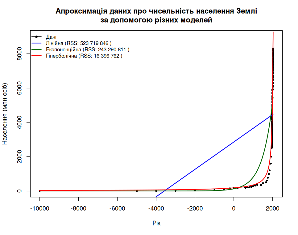
All that remains is to create a clear visualization. First, it is convenient to create sequences of evenly distributed points.


t_seq <- seq(min(t), max(t), length.out = 500)
pred_lin <- predict(fit_lin, newdata = list(t = t_seq))
pred_exp <- predict(fit_exp, newdata = list(t = t_seq))
pred_hyp <- predict(fit_hyp, newdata = list(t = t_seq))

A clear legend will be needed.


legend_labels <- c(
  "Дані",
  paste("Лінійна (RSS:", format(round(rss_lin, 0), big.mark=" "), ")"),
  paste("Експоненційна (RSS:", format(round(rss_exp, 0), big.mark=" "), ")"),
  paste("Гіперболічна (RSS:", format(round(rss_hyp, 0), big.mark=" "), ")")    )

The visualization itself. We will use the basic properties of R.


plot(t, N_mil, 
     pch = 16, cex = 0.7, col = "black",
     main = "Апроксимація даних про чисельність населення Землі\nза допомогою різних моделей",
     xlab = "Рік", ylab = "Населення (млн осіб)",
     ylim = c(0, 9000))
lines(t_seq, pred_lin, col = "blue", lwd = 2)
lines(t_seq, pred_exp, col = "darkgreen", lwd = 2)
lines(t_seq, pred_hyp, col = "red", lwd = 2)
legend("topleft", 
       legend = legend_labels,
       col = c("black", "blue", "darkgreen", "red"), 
       lwd = 2, pch = c(16, NA, NA, NA),
       cex = 0.85, bty = "n")

growth