Biostatistics — 12. Topic 8. Cluster analysis

←

D.A. Shabanov, M.A. Kravchenko. Statistical analysis of data in zoology and ecology

→

Topic 7. The relationship between traits

Topic 8. Cluster analysis

Topic 9. Principal component analysis

Biostatistics-11

Biostatistics-12

Biostatistics-13

8.1. The essence of cluster analysis
Cluster analysis is the name given to various formalized procedures for constructing classifications of objects. The leading science in the development of cluster analysis was biology. The subject of cluster analysis (from the English "cluster" — a bunch, tuft, group) was formulated in 1939 by the psychologist Robert Tryon. The classics of cluster analysis are the American systematists Robert Sokal and Peter Sneath. One of their most important achievements in this field is the book "Principles of Numerical Taxonomy", published in 1963. According to the authors' main idea, a classification should be built not on a mixture of poorly formalized judgements about the similarity and kinship of objects, but on the results of the formalized processing of the mathematically computed similarities/differences of the classified objects. To accomplish this task, suitable procedures were needed, and the authors set about developing them.
The main stages of cluster analysis are as follows:
1. the selection of the objects to be compared with one another;
2. the selection of the set of traits by which the comparison will be carried out, and the description of the objects by these traits;
3. the computation of the measure of similarity between objects (or the measure of difference between objects) according to the chosen metric;
4. the grouping of objects into clusters by means of one or another joining procedure;
5. the checking of the suitability of the obtained cluster solution.
Thus, the most important characteristics of the clustering procedure are the choice of metric (in different situations a considerable number of different metrics are used) and the choice of the joining procedure (and in this case too a considerable number of different variants are available for choice). For different situations one or another metric and joining procedure is more suitable, but to a certain degree the choice between them is a matter of taste and tradition. As is explained in more detail in the article "Clusters, clades, and the chimera of objectivity", the hope that cluster analysis will lead to the construction of a classification that does not depend on the arbitrariness of the researcher turns out to be unattainable. Of the five listed stages of research using cluster analysis, only stage 4 is not connected with the making of a more or less arbitrary decision that influences the final result. The choice of objects, the choice of traits, and the choice of metric together with the joining procedure all substantially influence the final result. This choice may depend on many circumstances, in particular on the explicit and implicit preferences and expectations of the research. Unfortunately, the noted circumstance affects not only the result of cluster analysis. All "objective" methods face similar problems, including all the methods of cladistics.
Is there a single correct solution that must be found when choosing the set of objects, the set of traits, the type of metric, and the joining procedure? No. To prove this, let us cite a fragment of the article referred to in the previous paragraph.
"In fact, we cannot always even firmly answer the question of which objects are more similar to one another and which differ more strongly. Unfortunately, for the choice of a metric of similarity and difference between classified objects there simply are no generally accepted (let alone "objective") criteria.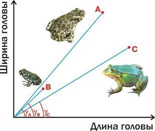
Chimaera 20
Which object is object A more similar to: B or C? If we use distance as the metric of similarity, then to C: |AC|<|AB|. But if we rely on the correlation between the traits shown in the figure (which can be described as the angle between the vector going to the object from the origin of coordinates and the abscissa axis), then to B: Chimaera 19 . And which is correct? There is no single correct answer. On the one hand, an adult frog is more similar to an adult frog (both adult), on the other — to a younger frog (both frogs)! The correctness of the answer depends on what we consider more important."
Cluster analysis has found wide application in modern science. Unfortunately, in a considerable part of the cases where it is used, it would be better to use other methods. In any case, biology specialists must clearly understand the basic logic of cluster analysis, and only in that case will they be able to apply it in those cases where it is adequate, and not apply it when the optimal choice is a different method.
8.2. An example of performing cluster analysis "on one's fingers"
To explain the typical logic of cluster analysis, let us consider a graphic example of it. Consider a set of 6 objects (denoted by letters), characterized by 6 traits of the simplest type: alternative ones, taking one of two values: characteristic (+) and non-characteristic (—). The description of objects by the adopted traits is called a "rectangular" matrix. In our case we are dealing with a 6×6 matrix, that is, it can be considered entirely "square", but in the general case the number of objects in the analysis may not equal the number of traits, and a "rectangular" matrix may have a different number of rows and columns. So, let us set a "rectangular" matrix (an objects/traits matrix):

—

The selection of objects and their description by a certain set of traits correspond to the first two stages of cluster analysis. The next stage is the construction of a matrix of similarity or difference (a "square" matrix, an objects/objects matrix). For this one must choose a metric. Since our example is conventional, it makes sense to choose the simplest metric. What is the simplest way to determine the distance between objects A and B? To count the number of differences between them. As you can see, objects A and B differ in traits 3 and 5, hence the distance between these two objects equals two units.
Using this metric, let us construct a "square" matrix (an objects/objects matrix). As is easy to verify, such a matrix consists of two symmetrical halves, and one can fill in only one of these halves:

—

In this case we have constructed a matrix of differences. A matrix of similarities would look similar, only at each position there would stand a value equal to the difference between the maximum distance (6 units) and the difference between the objects. For the pair A and B, naturally, the similarity would amount to 4 units.
Which two objects are closest to one another? B and F, they differ in only one trait. The essence of cluster analysis lies in the joining of similar objects into a cluster. We join objects B and F into a cluster (BF). We show this on the diagram. As you can see, the objects are joined at the level that corresponds to the distance between them.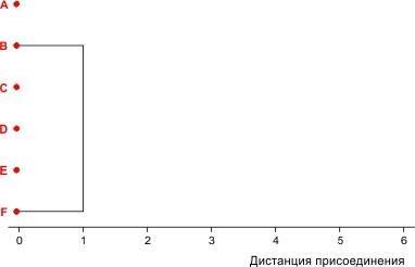

Fig. 8.2.1. The first step of clustering the conventional set of 6 objects
Now we have not six objects but five. We rebuild the "square" matrix. For this we need to determine the magnitude of the distance from each object to the cluster. The distance from A to B was 2 units, and from A to F — 3 units. What is the magnitude of the distance from A to (BF)? There is no correct answer here. Here, look at how these three objects are arranged relative to one another.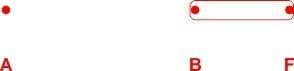

Fig. 8.2.2. The mutual arrangement of three objects
It may be that the distance from an object to a group is the distance from the object to the object nearest to it within the group, that is │A(BF)│=│AB│? Such logic corresponds to joining by maximum similarity.
Or it may be that the distance from an object to a group is the distance from the object to the object most distant from it within the group, that is │A(BF)│=│AF│? Such logic corresponds to joining by minimum similarity.
One may also consider that the distance from an object to a group is the arithmetic mean of the distances from this object to each of the objects within the group, that is │A(BF)│=(│AB│+│AF│)/2. This solution is called joining by average similarity.
All these three solutions are correct, and so is a considerable number of other solutions not characterized here. Our task is to choose the solution more suitable for the category to which our data belong. Joining by maximum similarity leads, in the final analysis, to long, "ribbon-like" clusters. By minimum — to the fragmentation of groups. Choosing among the three characterized variants, in biology joining by average similarity is more often used. We too shall make use of it. In that case, after the first step of clustering the "square" matrix will look like this.

(BF)

—

2.5

(BF)

—

3.5

2.5

—

Now the closest pair of objects is D and E. Let us join them too.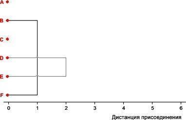

Fig. 8.2.3. The second step of clustering the conventional set of 6 objects
Let us rebuild the "square" matrix for four objects.

(BF)

(DE)

—

2.5

(BF)

—

3.5

2.5

—

(DE)

—

We see that here there are two possibilities for joining at the level of 2.5: the joining of A to (BF) and the joining of (BF) to (DE). Which of them to choose?
We have various options for how to make such a choice. It can be made at random. One can adopt some formal rule that allows the choice to be made. Or one can look at which of the solutions gives the better clustering variant. Let us use the last option. First let us realize the first variant.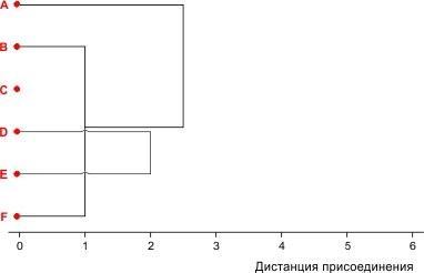

Fig. 8.2.4. The first variant of the third step of clustering the conventional set of 6 objects
Having chosen this variant, we would have had to construct the following "square" 3×3 matrix.

(ABF)

(DE)

(ABF)

—

3.25

—

(DE)

—

If we had chosen the second variant of the third step, we would have got the following picture.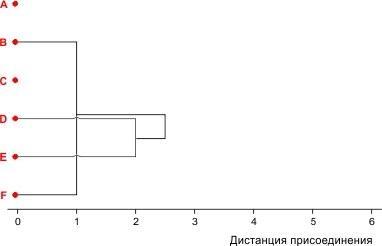

Fig. 8.2.5. The second variant of the third step of clustering the conventional set of 6 objects
It corresponds to the following 3×3 matrix:

(BFDE)

—

3.25

—

(BFDE)

—

The obtained 3×3 matrices can be compared, and one can verify that a more compact group of objects is achieved in the second variant. In constructing a classification of objects by means of cluster analysis, we must strive to single out groups that unite similar objects. The higher the similarity of objects within groups, the better such a classification. Therefore we choose the second variant of the third step of clustering. Of course, we could have taken further steps (and split the first variant into two more subvariants), but in the final analysis we would have become convinced that the best variant of the third step of clustering is precisely the one shown in Fig. 8.5. We settle on it.
In that case the next step is the joining of objects A and C, shown in Fig. 8.6.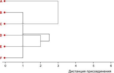

Fig. 8.2.6. The fourth step of clustering
We construct a 2×2 matrix:

(AC)

(BFDE)

(AC)

—

3.625

(BFDE)

—

Now there is no longer anything to choose. We join the two remaining clusters at the required level. In accordance with the adopted style of constructing cluster "trees", we add one more "trunk", which extends to the level of the maximum distance between objects possible with the given set of traits.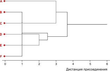

Fig. 8.2.7. The fifth and last step of clustering
The obtained picture is a tree-like graph (a set of vertices and links between them). This graph is constructed so that its lines intersect (we have marked these intersections with "little bridges"). Without changing the character of the links between objects, the graph can be rebuilt so that there are no intersections in it at all. This is done in Fig. 8.2.8.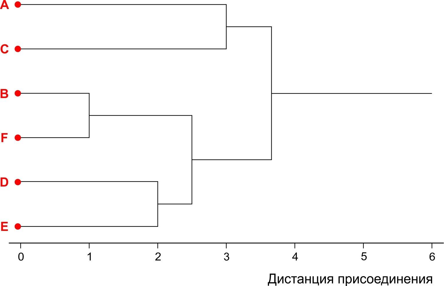

Fig. 8.2.8. The final appearance of the tree-like graph obtained as a result of clustering
The cluster analysis of our conventional example is complete. It remains only for us to understand what exactly we have obtained.
8.3. Fundamental limitations and shortcomings of cluster analysis
How is the graph shown in Fig. 8.2.8 to be interpreted? There is no unambiguous answer. To answer this question, one must understand which data and with what aim we clustered. "On the surface" lies the conclusion that we have established that the initial set of 6 objects consists of three pairs. Looking at the obtained graph, it is hard to doubt this. However, is this conclusion valid?
Return to the first "square" 6×6 matrix and verify: object E was at a distance of two units both from object D and from object F. The similarity of E and D is reflected in the final "tree", but the fact that object E was just as close to object F — has vanished without a trace! How is this to be explained?
In the result of clustering shown in Fig. 8.2.8, information about the distance │EF│ is completely absent; there is only information about the distances │DE│ and │(BF)(DE)│!
To each "rectangular" matrix, in the case when a certain metric and method of joining have been chosen, there corresponds one single "square" matrix. However, to each "square" matrix many "rectangular" matrices may correspond. After each step of the analysis, to each preceding "square" matrix there corresponds the next one, but, proceeding from the next one, we would not be able to restore the previous one. This means that at each step of cluster analysis a certain part of the information about the diversity of the initial set of objects is irreversibly lost.
The noted circumstance is one of the serious shortcomings of cluster analysis.
One more of the insidious shortcomings of cluster analysis is mentioned in the article "Lies, damned lies, and…", in the section "Misunderstanding the essence of the method".