Gauss – I believe!

The publication of a blog post devoted to elections turned out to be instructive for me—it provoked an unexpectedly broad and emotional reaction. I even began it with the claim that different things are convincing for different people. Since static distributions turned out to be very convincing for me, I wrote that post. The next step was its discussion, both in the comments and on my website. The picture of the discussion made me dream of another way of processing data. Imagine: we take a sufficiently rich debate on some internet platform and compare the supporters of two points of view in terms of literacy, logical consistency, and formal politeness of their texts. Of course, unbiased methods for evaluating the necessary textual parameters are needed… However, without any statistical apparatus such a analysis is carried out by any attentive reader who follows online discussions. It ended like this. I answered the objections that seemed substantial to me. Many comments remained unanswered. By “points” (the number of contributions) I lost. In fact, I was convinced of my correctness and, I hope, managed to persuade many reasonable readers. Unfortunately, it seemed to me that many of us simply lack an understanding of the basics of statistics. I will try to explain a bit more clearly. And I will start with a 10‑mark banknote issued at a time when Germany had not yet adopted the euro. Figure 1. Someone will first see here a foreign currency sign with a culture alien to many Russians. Such (or newer) notes are sold by liberals alien to the Russian spirit!

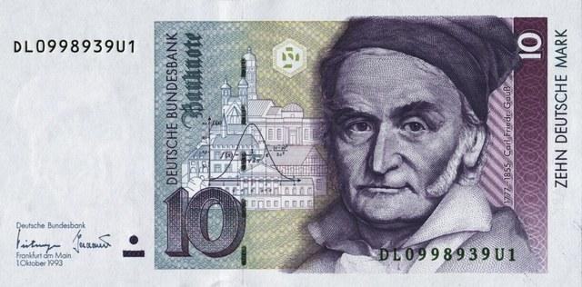
The banknote bears a portrait of Carl Gauss, an equation and a graph of the Gaussian. Money is just money, an economic symbol. To make people trust these notes, references to some foundation are sewn into them—both to the national bank, to science, and to culture. It is not the authority of money that supports mathematics; it is a classic of mathematics that supports the authority of money! What is so unusual about the normal, Gaussian distribution? The fact that a quantity influenced by many independent factors has a distribution that tends toward normality. Look, for example. I generate an array of 10 random variables whose distributions are shown in the figure, and compute 500 values. Figure 2. Along the diagonal are the distributions of 10 random variables ranging from 0 to 1 (500 values each).

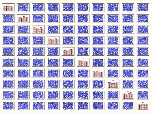
At the intersections of the horizontal and vertical lines extending from the diagonal are two‑dimensional point distributions showing the lack of correlation between the variables. Now we sum these quantities. The distribution of the sum is close to normal. The mean is 5, but in no case does the sum equal, for instance, 1 or 9. Those values are possible but extremely unlikely. Figure 3.

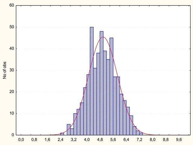
Almost a miracle. The sum of 10 uniformly distributed random variables acquired a normal distribution. The most probable value is 5. In fact, we simply illustrated the central limit theorem. We saw that in this case the distribution of sums of independent random variables was close to normal, and the theorem proves this circumstance! What happens if one of the factors turns out to be obviously stronger than the others?

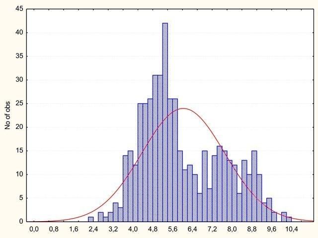
Let us add an eleventh factor to the sum: in one‑third of cases it equals 3, in two‑thirds it equals 0. Figure 4. To the sum whose distribution is shown in the previous graph, an additional term has been added. In two‑thirds of cases we added nothing, and in one‑third we added 3. The distribution acquired a right‑skewed “tail.” By the way, what if we added 3 to all cases? The curve would simply shift three units to the right, and the average result would be 8. Thus, the “tail” of the distribution indicates the presence of a powerful factor that does not act in all cases. We have confirmed some properties of the normal distribution. Now let us model conditional elections. At this stage we use the following simplifications: each polling station is assigned 3 000 voters; 49 % of voters vote for party 1, 19 % for party 2, 13 % for party 3, 12 % for party 4, 3 % for party 5, 0.3 % for party 6, and 5.7 % for the remaining parties; for each voter the probability of reaching the polling station is the same (60 %); the party a voter chooses does not depend on whether he/she comes to the station, which station he/she goes to, how many people voted at that station, or how the votes are distributed. Clearly, such a model is much simplified compared with reality. It is implemented as follows. In the program Statistica‑7, 150 000 “voters” are defined (500 stations × 3 000 votes per party). Each of them votes for party 1 with probability 0.49 and for the other parties with the corresponding probabilities; each of them reaches the station with probability 0.6. Turnout at the stations varied somewhat. Are you surprised that this variable is bell‑shaped? Figure 5. Distribution of polling stations in the model “election” by the number of voters who turned out (each voter arrived at the station with probability 0.6).

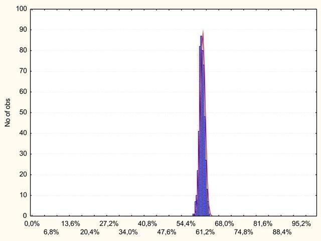
And how did the votes for the parties distribute? Let us see the result. Figure 6.

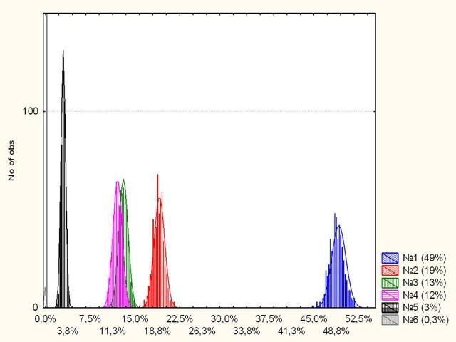
Distribution of votes for six parties in the model “election.” All distributions are bell‑shaped except for the one of the least popular party (0.3 %). Apparently, we need to look more closely at the distribution of votes for the smallest party.

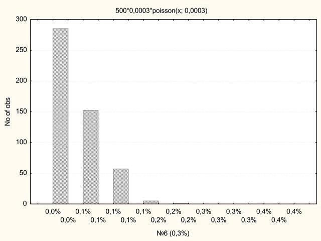
Figure 7. Party 6 received 0.3 % of the votes. Its distribution is Poisson. This Poisson distribution is the distribution of the number of coincidences of independent rare events. As you can see, on most stations nobody voted for this party. What would happen if the probability of votes for a certain party increased? As the probability of votes for a party rises, the peak of the distribution will detach from zero, will crawl away from zero, and the Poisson distribution will transition to a distribution close to normal (bell‑shaped). As the party’s popularity grows, this distribution will retain its bell‑shaped character as long as the probability of voting for it remains sufficiently substantial. And what about those readers who claimed that all distributions except the one for the party that received the maximum votes should be close to normal? Nonsense. And why “close to normal” rather than “normal”? Because each additional vote for a given party not only increases the percentage of votes for it but also raises turnout, reducing the “weight” of all previous votes. I will not delve into statistical subtleties now; answering the critics who consider this distribution log‑normal (the logarithm of a normal), I will say that in such cases the difference between these distributions is negligible. Figure 8. This is the distribution of votes for the leading party on a larger scale. In the discussion of the previous post about elections many copies were broken on the issue of whether to associate a normal or a log‑normal distribution with the votes for a party. The answer: practically no difference!

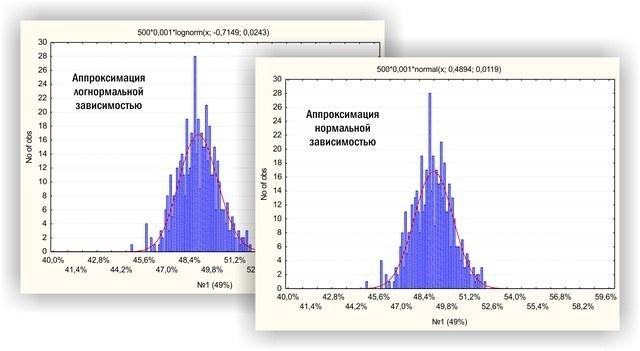
At what turnout do deviations from normality become more serious: with constant or variable turnout? Many readers of my previous post argued that variable turnout is the cause of the statistical effects registered in the analysis of Russian election results. Fine, let us see how variable turnout affects vote distributions. Figure 9. Distribution of 500 stations by turnout. The maximum is 100 % turnout, 3 000 votes (compare with Fig. 5).

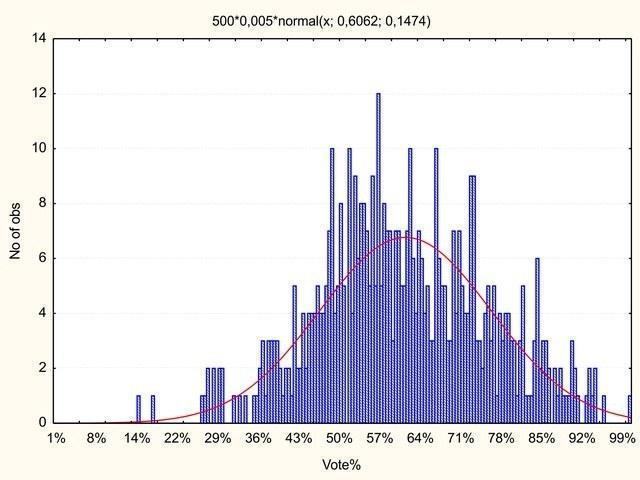
So what changed? Figure 10.

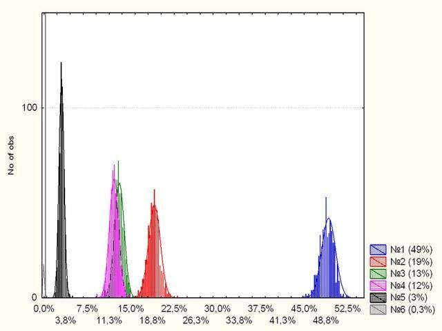
Distribution of votes for six parties with variable turnout. Compare with Fig.

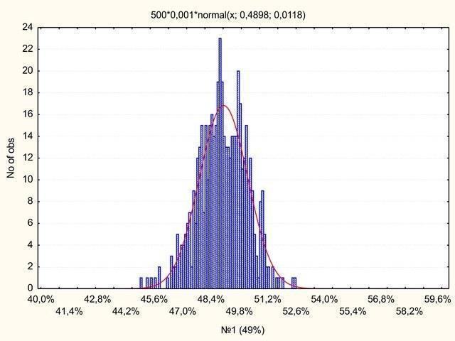
6: virtually nothing changed. Let us look more closely at the leading party… Figure 11. Distribution of votes for the leading party with variable turnout (compare with Fig. 8).

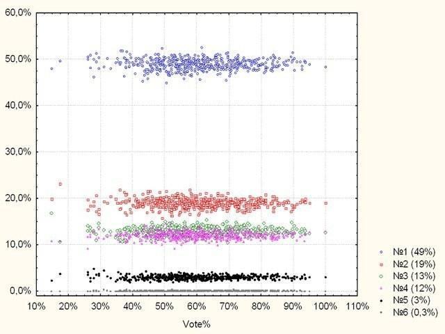
The same story. Finally, the last point. Among the objections to the statistical methods used to analyse the results was the idea that as turnout rises, the percentage of votes for the most numerous party should also rise. See. Figure 12. Dependence of the results for six parties on overall turnout at stations. The share of votes remains constant (assuming that each voter’s preferences are formed independently of turnout at his/her station). So far we have not been talking about the Russian elections of December this year, but about a simple model of them. We have shown that if the result of an election at each station is influenced by many independent events (the voting decisions of many independent citizens), the resulting distributions are bell‑shaped and close to normal. This model differs markedly from reality because it uses truly independent votes. Each voter does not vote randomly; he/she may have systematic reasons for certain preferences. But if the decisions made by voters are independent of the decisions of other voters and of turnout at the station, the resulting distributions are fully Gaussian. Sometimes “tails” and bimodality of distributions turn out to be linked to the mixing of two (or more) heterogeneous samples (for example, stations in a city and in a village or in regions with different social conditions). This is a fact that does not depend on anyone’s decision. Yet the hypothesis of such a distributional character can be tested by examining the statistics for groups of heterogeneous stations separately. How does a successful campaign affect a party’s result? It raises the probability that a voter will give a vote to that party. The distribution of votes across stations remains bell‑shaped but shifts toward higher values. How does ballot stuffing in favour of a party affect its result? Roughly as in Fig. 4: it creates a pronounced “tail.” The space allotted to me has long been exhausted. I will formulate a hypothesis. All legal methods of political struggle do not lead to a substantial deviation of the considered distributions from normality. A significant portion of the measures used in election fraud or administrative influence on the process leads to deviations from bell‑shaped distributions and the formation of “tails” in the samples. If you wish, I will continue.