Creation of Worlds — 08. R as an Environment for Simulation Modelling

8. R as an environment for simulation modelling
8.1. Exponential and logistic growth of a model population
Every tool has its own specifics. Of course, both LO Calc and R can be used to implement the same conceptual models. In this online textbook we will begin with exactly that: we will replicate some of the models whose construction is explained in detail for LO Calc. Even at this stage an important advantage of R will become apparent. To create a model in this programming language, a few lines of code — scripts — will sometimes suffice. Once you have mastered R, you will realise that this language opens up far broader possibilities for simulation modelling. LO Calc is an amateur tool whose advantage lies in its low entry threshold. R is already a genuinely professional tool. In some respects it may lag behind possible professional alternatives, while in others (for example, in the diversity of packages for statistical analysis) it has no equal. Of course, once you have mastered modelling in R, your working style with models will change substantially, and your capabilities will expand immeasurably.
In this course we will not spend time introducing R. Students who studied at the undergraduate level in the Department of Zoology and Animal Ecology at V. N. Karazin Kharkiv National University were required to take a course in data analysis in zoology and ecology; that is where their introduction to the R language and environment was supposed to occur. Links to pages covering the basics of working with R can be found on this page, at the top, below the panel that provides navigation within the course. The library available on this website may also be useful. Where to obtain the R and RStudio installers, and what to do with them, is already described in the relevant section of the "Statistical Oracle".
As in this course as a whole, we will begin with the exponential model, to which the entire second chapter is devoted. The model is, of course, very simple, but it serves as a convenient example for learning to work with LO Calc. R-dialogue 8.1 shows how this model can be implemented using R.
R-dialogue 8.1. Example of a simple model in R: exponential growth

> > # Exponential growth of a model population
> initial <- 1000 # Initial population size 
> r <- 0.1 # Malthus parameter (biotic potential)
> t <- 50 # Number of simulation steps
> dynamics <- (0:t) # Create a vector for the results
> N <- initial # The first value of the population size
> dynamics[1] <- initial # The first value is set differently from the following ones
> for (i in 2:(t+1)) { # Start of the loop for step-by-step filling of the vector
+ + # The count i starts at 2 because the first value of the dynamics vector is the initial value!
+   N <- N + N*r # Exponential growth formula
+   dynamics[i] <- N # Step-by-step storing of the results
+ } # End of the loop
> plot(dynamics) # The simplest visualization
> dynamics # Print the resulting vector to the console
 [1]   1000.000   1100.000   1210.000   1331.000   1464.100   1610.510   1771.561   1948.717   2143.589   2357.948
[11]   2593.742   2853.117   3138.428   3452.271   3797.498   4177.248   4594.973   5054.470   5559.917   6115.909
[21]   6727.500   7400.250   8140.275   8954.302   9849.733  10834.706  11918.177  13109.994  14420.994  15863.093
[31]  17449.402  19194.342  21113.777  23225.154  25547.670  28102.437  30912.681  34003.949  37404.343  41144.778
[41]  45259.256  49785.181  54763.699  60240.069  66264.076  72890.484  80179.532  88197.485  97017.234 106718.957
[51] 117390.853
> 

When dealing with the model shown in R-dialogue 8.1, one must bear in mind that the length of the results vector is one greater than the number of model steps. The first value in this vector corresponds to the initial, "zeroth" value; the second corresponds to the value after the first simulation step, and so on. If, as in most programming languages, the first value in R had index 0, this would be quite convenient. However, the R language implements a common-sense variant — in it, the first value has index 1. Examine Fig. 8.1: the last value of the model population size, computed after the fiftieth model step, is the fifty-first.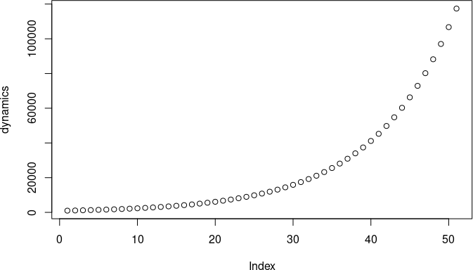

Fig. 8.1. The graph produced by the script shown in R-dialogue 8.1.
In some cases this offset may be inconvenient. Think of a way to correct it!
The next step is the logistic model. When constructing it, the experience gained from the exponential model should be taken into account (R-dialogue 8.2).
R-dialogue 8.2. Model implementing logistic growth with probabilistic rounding

> R-dialogue 8.2. Model implementing logistic growth with probabilistic rounding
> N <- 1000 # Initial size
> r <- 0.03 # Malthus parameter (biotic potential)
> K <- 10000 # Verhulst parameter (carrying capacity of the environment)
> t <- 400 # Number of simulation steps
> Dynamics <- (0:t) # Vector with the population size
> Steps <- (0:t) # Vector - a step counter
> Dynamics[1] <- N # Initial value 
> for (i in 2:(t+1)) { # Start of the loop
+   N <- floor(N + N*r*(K-N)/K + runif(1, min = 0, max = 1)) Probabilistic rounding
+   Dynamics[i] <- N # Step-by-step storing of the results
+ } # End of the loop
> plot(Steps, Dynamics) # Dependence of the values of one vector on the values of another
> Dynamics[t+1] # The last value of the population-size vector
[1] 9999
> 

In this case we output to the console not the entire sequence of population size values, but only the last value. A question arises: if the carrying capacity equals 10,000, why is the value reached at step 400 only 9,999? The issue is not that the model population has not had time to reach the growth limit, since its graph shows that the model population size stabilised long before the end of the simulation (Fig. 8.2). What, then, is the reason?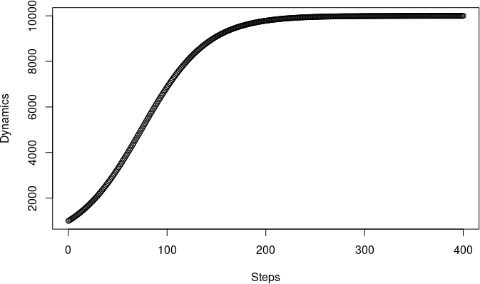

Fig. 8.2. Logistic growth produced by the script shown in R-dialogue 8.2.
Incidentally, if you run the model shown in R-dialogue 8.2, the last value in the Dynamics vector will not necessarily be 9,999. Why?
As you can see, the model under discussion does not account for mortality of individuals that have reached a certain age, as was done in section 3.2. Age-specific mortality. Write a model that takes this into account on your own! Of course, you will have to remember that population size cannot be negative.
8.2. The "Three-Generation Model"
When studying modelling with LO Calc, the first barrier that students often find difficult to overcome is the model that considers the demographic structure of a population. Using this model as an example, LO Calc users are introduced to the typical structure of a simulation model: a table in which columns are variables and rows are simulation cycles. In the course, this model is the first to use many "adult" (in reality, of course, "adolescent") features of design and operation. The same conceptual model reflected in the LO Calc model discussed in this course can be implemented in R in different ways. We will first consider a version of the model that is practically identical to what was constructed in LO Calc. In this case we will not present a console dialogue, but will simply include the R script in the text. We will do this quite often from here on. R scripts will be distinguished from the surrounding text by their font (R-script 8.1).
R-script 8.1. The "Three-Generation Model" in a form that duplicates the structure of its LO Calc implementation

> <...>
> colnames(Competitions) <- Groups 
> set.seed(33333) # This command makes the random numbers the same on repeated runs
> for (i in 1:t){
+ BetaNumber <- floor(AlphaNumber * Surviv + runif(1, min = 0, max = 1)) # Beta abundances
+ print("i")
+ print(i)
+ print("BetaNumber")
+ print(BetaNumber)
+ GammaNumber <- BetaNumber * Compet 
+ print("GammaNumber")
+ print(GammaNumber)
+ <...>
+ om_O_f0 <- floor(om_O * p_f + runif(1, min = 0, max = 1)) 
+ om_O_m0 <- om_O - om_O_f0
+ print(om_O)
+ print(om_O_f0)
+ print(om_O_m0)
+ AlphaNumber <- c(om_O_f0, DeltaNumber[1], DeltaNumber[2], om_O_m0, DeltaNumber[4], DeltaNumber[5])
+ } 
[1] "i"
[1] 1
[1] "BetaNumber"
[1] 14  4  1  7  1  0
[1] "GammaNumber"
[1] 8.4 2.8 0.8 4.9 0.8 0.0
[1] "DeltaNumber"
[1] 14  4  1  7  1  0
[1] 2
[1] 2
[1] "i"
[1] 2
[1] "BetaNumber"
[1]  2 12  3  2  5  1
[1] "GammaNumber"
[1] 1.2 8.4 2.4 1.4 4.0 0.9
[1] "DeltaNumber"
[1]  2 12  3  2  5  1
[1] 18
[1] 12
<...>
> 

al1_n_f1 <- 16 # Initial number of first-age females
al1_n_m1 <- 10 # Initial number of first-age males
K <- 50 # Carrying capacity
b_f2 <- 3 # Fecundity of second-age females
b_f3 <- 15 # Fecundity of third-age females
om_T <- 2 # Number of females a single male can fertilise
p_f <- 0.7 # Proportion of females in offspring
t <- 50 # Number of simulation cycles
VarNames<-c("al_n_f1", "al_n_f2", "al_n_f3", "al_n_m1", "al_n_m2", "al_n_m3", "al_N", "be_Q", "be_n_f1", "be_n_f2", "be_n_f3", "be_n_m1", "be_n_m2", "be_n_m3", "om_N_F", "om_N_M", "om_P_f2", "om_P_f3", "om_O", "om_n_f0", "om_n_m0")
G3 <- matrix(NA, nrow = t+1, ncol = length(VarNames))
colnames(G3) <- VarNames # Column names are variable designations chosen according to the general principles of the course
rownames(G3) <- 0:t # Matrix rows are simulation cycles
G3[1,"om_n_f0"] <- al1_n_f1 # Offspring (omega-abundance) in row "0" will determine...
G3[1,"om_n_m0"] <- al1_n_m1 # ...the alpha-abundance of first-age individuals in row "1"
G3[1,"be_n_f1"] <- 0 # Beta-abundance of first-age individuals in row "0" will determine...
G3[1,"be_n_m1"] <- 0 # ...the alpha-abundance of second-age individuals in row "1"
G3[1,"be_n_f2"] <- 0 # Beta-abundance of second-age individuals in row "0" will determine...
G3[1,"be_n_m2"] <- 0 # ...the alpha-abundance of third-age individuals in row "1"
for (a in 1:t){ i <- a + 1 # At the start i=1 corresponding to row "0", and a=2 corresponding to row "1"
G3[i,"al_n_f1"] <- G3[a,"om_n_f0"] # Alpha-abundances...
G3[i,"al_n_f2"] <- G3[a,"be_n_f1"] # ...of the next cycle...
G3[i,"al_n_f3"] <- G3[a,"be_n_f2"] # ...are set on the basis of...
G3[i,"al_n_m1"] <- G3[a,"om_n_m0"] # ...omega-abundances...
G3[i,"al_n_m2"] <- G3[a,"be_n_m1"] # ...and beta-abundances...
G3[i,"al_n_m3"] <- G3[a,"be_n_m2"] # ...of the previous cycle
G3[i,"al_N"] <- G3[i,"al_n_f1"] + G3[i,"al_n_f2"] + G3[i,"al_n_f3"] + G3[i,"al_n_m1"] + G3[i,"al_n_m2"] + G3[i,"al_n_m3"]
ifelse(G3[i,"al_N"]<=K, G3[i,"be_Q"] <- 1, G3[i,"be_Q"] <- K / G3[i,"al_N"]) # Condition written concisely on one line
G3[i,"be_n_f1"] <-floor(G3[i,"al_n_f1"] * G3[i,"be_Q"] + runif(1, min = 0, max = 1)) # Beta-...
G3[i,"be_n_f2"] <-floor(G3[i,"al_n_f2"] * G3[i,"be_Q"] + runif(1, min = 0, max = 1)) # ...abundances...
G3[i,"be_n_f3"] <-floor(G3[i,"al_n_f3"] * G3[i,"be_Q"] + runif(1, min = 0, max = 1)) # ...are computed...
G3[i,"be_n_m1"] <-floor(G3[i,"al_n_m1"] * G3[i,"be_Q"] + runif(1, min = 0, max = 1)) # ...using...
G3[i,"be_n_m2"] <-floor(G3[i,"al_n_m2"] * G3[i,"be_Q"] + runif(1, min = 0, max = 1)) # ...probabilistic...
G3[i,"be_n_m3"] <-floor(G3[i,"al_n_m3"] * G3[i,"be_Q"] + runif(1, min = 0, max = 1)) # ...rounding
G3[i,"om_N_F"] <- G3[i,"be_n_f2"] + G3[i,"be_n_f3"] # Total number of mature females
G3[i,"om_N_M"] <- G3[i,"be_n_m2"] + G3[i,"be_n_m3"] # Total number of mature males
if(G3[i,"om_N_F"]==0) # Check in case no mature females are present
{G3[i,"om_P_f2"] <- 0 # When computing the number of pairs with second- and third-age females...
G3[i,"om_P_f3"] <- 0} # ...division by the total number of mature females is required
else # This is the general case when mature females are present
{if(G3[i,"om_N_F"]/G3[i,"om_N_M"] > om_T) # If males are insufficient, they limit the number of pairs
{G3[i,"om_P_f2"] <-round(G3[i,"om_N_M"] * om_T * G3[i,"be_n_f2"] / G3[i,"om_N_F"])
G3[i,"om_P_f3"] <-round(G3[i,"om_N_M"] * om_T * G3[i,"be_n_f3"] / G3[i,"om_N_F"])}
else # If males are sufficient, the number of pairs is limited by the number of mature females
{G3[i,"om_P_f2"] <-G3[i,"be_n_f2"]
G3[i,"om_P_f3"] <-G3[i,"be_n_f3"] } # Closing brace of the else that determines who limits the number of pairs
} # Closing brace of the else that determines whether females are present
G3[i,"om_O"] <- G3[i,"om_P_f2"] * b_f2 + G3[i,"om_P_f3"] * b_f3 # Number of offspring
G3[i,"om_n_f0"] <-floor(G3[i,"om_O"] * p_f + runif(1, min = 0, max = 1)) # Females in offspring
G3[i,"om_n_m0"] <-G3[i,"om_O"] - G3[i,"om_n_f0"] # Males in offspring
} # Closing brace of the for loop that counts matrix rows
ThreeGenerations <- G3[-1,] # Row named "0" is removed from the file
head(ThreeGenerations, 3) # Preview of the first three rows of the resulting file
tail(ThreeGenerations, 3) # Preview of the last three rows of the resulting file
par(lwd=2, cex=0.9, font.lab=1) # Graphics parameters: line width, font size, font type
plot(ThreeGenerations[,"om_N_F"], type="l", lty=1, col="red", # First line, its type, character, and colour
main="Population dynamics of mature individuals in the Three-Generation Model", # Title
xlab="Simulation cycles", ylab="Abundance") # Axis labels
lines(ThreeGenerations[,"om_N_M"], type="l", lty=5, col="blue") # Second line
legend("topright", inset=.05, title="Legend", c("Females","Males"), # Legend
lty=c(1, 2), col=c("red", "blue")) # Compared elements in the legend

Input parameters are set in lines 1-8.
In lines 9-11 a matrix for the output data is created. At the moment of creation this matrix is empty; its cells are filled with NA. It has 21 columns (many, of course...) and one more row than the number of cycles specified in the input parameters. The reason is that the first row, which will receive a name (not a number; the number will be 1), will serve to record the initial abundances.
Lines 13-18: Filling the row named "0" (the 1st by count) with initial data.
Lines 19 to 50: The main loop, which sequentially counts matrix rows and fills them.
Lines 20-25: computation of alpha-abundances. In the row named "1" with number 2 (at the end of the script it will receive number 1), the first 6 cells are filled.
Line 26: alphaaN is determined.
Line 27, which uses the ifelse condition written concisely on one line — betaQ is calculated.
Lines 28-33: beta-abundances.
Lines 34-49: computation of offspring. First (34, 35) the abundance of both sexes is computed.
The first if-else condition (lines 36-46) checks whether there are any females at all; if there are, a second condition appears in the computations (lines 40-45), which determines which sex limits the number of broods.
In line 51 the matrix G3, with which we have been working up to this point, is transformed into the matrix ThreeGenerations. For this it is sufficient to discard from G3 the first (by count) row, which contained the initial abundance values for all 6 groups.
Lines 52 and 53 allow the result to be viewed in the console.
Lines 54-60: description of the graph. The graph has two lines; consequently, the coordinate axes are first constructed with the first line, and then a second is added.
Execution of the final part of this script, which is responsible for building the graph, produces the image shown in Fig. 8.3. It is important that the population dynamics in two different implementations (in LO Calc and in R) of the same conceptual model are identical; differences arise from the fact that both models are non-deterministic owing to probabilistic rounding to integers.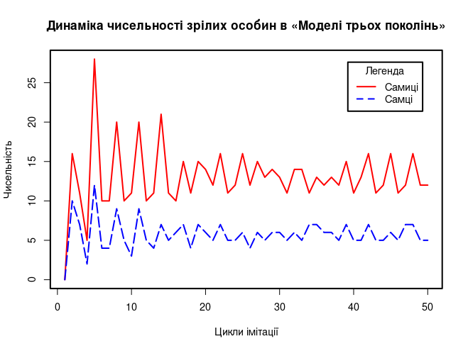

Fig. 8.3. The graph produced by R-script 8.1.
However, an important question arises. Must the organisation of a model in R always duplicate its organisation in LO Calc?
Clearly the answer to the preceding question must be negative. Every tool has its own specifics. First of all, bear in mind that most cells in the LO Calc implementation of the model shown in Fig. 4.1 are not examined by the user. This is more clearly visible in Fig. 4.10: there is a field of fairly extensive computations, while only 2-3 columns containing various integral indicators of dynamics go to the "output" graph. And what purpose do these cells serve in the model?
The first reason is that the "additional" cells reduce the number of computations. Let us illustrate this with the Three-Generation Model. Suppose we need to transition from alpha-abundance to beta-abundance. For this, a reduction coefficient betaQ is used. In combined notation betaQ=IF(alphaN>K;K/alphaN;1). After this, in the following 6 columns this result is used to compute the beta-abundances: betansa=ROUNDDOWN(alphansa x omegaO+RAND();). Of course, this column could have been omitted, and the calculation betansa=IF(alphaN>K;ROUNDDOWN(alphansa x K/alphaN+RAND(););alphansa) could simply have been repeated six times. Yet another column (and a cell in each cycle) contains the recalculation of alphaN. Into the six beta-abundance calculations one could have inserted the formula for computing alphaN as the sum of all alpha-abundances... That would have been a poor decision. It would have resulted in the same computations being performed six times per cycle instead of once. Moreover, it would have made the formulas far more cumbersome; the consequence would have been a significantly greater likelihood of error when writing them, and significantly greater effort required for checking them during model debugging. And this brings us to the second reason why it is desirable to break computations into separate steps.
The second reason is that searching for errors in the model is an almost essential stage of the work. The typical task — when the final result of the computations is not as required (produces an error, or is absurd from some standpoint) — is to find the point in the model where its operation went wrong. The more detailed the representation of intermediate computations, the easier it is to find the cell after which the operation diverged from what was intended. What justifies the presence of "additional" cells is that they simplify understanding of the model.
Let us also give a third reason. In reality, a model must not only establish what consequences follow from a given set of initial parameters and conditions; it must persuade the user and "observers" of this (for example, readers of a paper presenting the modelling results). When all stages of the computations are transparent, it is easier to understand how the model works.
Do these reasons apply to R? The first — unquestionably. The second — does not require saving all intermediate computation results, since they can be called up at any time if necessary. To this end, during verification of the model's operation, a command can be inserted at any point in the script that will output any stage of the computations to the console. When it is needed, we call it; when it is not needed, it need not be shown. As for transparency, it may be noted that a substantial difference exists between models in spreadsheets and models in R. R models are not comprehensible at first glance, but, for example, their scripts can be included in papers or reports. When you look at a model in a spreadsheet, you cannot be certain that all formulas in it work as intended; R models are more "transparent" and easier to verify.
As a result of these and other reasons, the following variant often proves optimal for R models. During the simulation, only the key variables can be saved in the output file — that is, those indicators used for the final visualisation or concluding computations. All intermediate results that can be reproduced from the key indicators need not be stored. Let us try to rework the model shown in R-script 8.1 in this way (R-script 8.2).
R-script 8.2. The "Three-Generation Model": a condensed version

al1_n_f1 <- 16 # Initial number of first-age females
al1_n_m1 <- 10 # Initial number of first-age males
K <- 50 # Carrying capacity
b_f2 <- 3 # Fecundity of second-age females
b_f3 <- 15 # Fecundity of third-age females
om_T <- 2 # Number of females a single male can fertilise
p_f <- 0.7 # Proportion of females in offspring
t <- 50 # Number of simulation cycles
VarNames<-c("n_f1", "n_f2", "n_f3", "n_m1", "n_m2", "n_m3")
ThreeGenerations <- matrix(NA, nrow = t, ncol = length(VarNames))
colnames(ThreeGenerations) <- VarNames # Column names are variable designations chosen according to the general principles of the course
om_n_f0 <- al1_n_f1 # Offspring (omega-abundance) will determine...
om_n_m0 <- al1_n_m1 # ...the alpha-abundance of first-age individuals in the next cycle
be_n_f1 <- 0 # Beta-abundance of first-age individuals will determine...
be_n_m1 <- 0 # ...the alpha-abundance of second-age individuals in the next cycle
be_n_f2 <- 0 # Beta-abundance of second-age individuals will determine...
be_n_m2 <- 0 # ...the alpha-abundance of third-age individuals in the next cycle
for (i in 1:t){ # Beginning of the main loop
al_n_f1 <- om_n_f0 # Alpha-abundances of the next cycle...
al_n_f2 <- be_n_f1 # ...are set on the basis of omega-abundances...
al_n_f3 <- be_n_f2 # ...and beta-abundances of the previous cycle...
al_n_m1 <- om_n_m0 # ...(or, in the case of the first simulation cycle —...
al_n_m2 <- be_n_m1 # ...those set before the start
al_n_m3 <- be_n_m2 # ...of the main computation loop defined by the for operator)
al_N <- al_n_f1 + al_n_f2 + al_n_f3 + al_n_m1 + al_n_m2 + al_n_m3
ifelse(al_N<=K, be_Q <- 1, be_Q <- K / al_N) # Condition on one line
be_n_f1 <-floor(al_n_f1 * be_Q + runif(1, min = 0, max = 1)) # Beta-...
be_n_f2 <-floor(al_n_f2 * be_Q + runif(1, min = 0, max = 1)) # ...abundances...
be_n_f3 <-floor(al_n_f3 * be_Q + runif(1, min = 0, max = 1)) # ...are computed...
be_n_m1 <-floor(al_n_m1 * be_Q + runif(1, min = 0, max = 1)) # ...using...
be_n_m2 <-floor(al_n_m2 * be_Q + runif(1, min = 0, max = 1)) # ...probabilistic...
be_n_m3 <-floor(al_n_m3 * be_Q + runif(1, min = 0, max = 1)) # ...rounding
ThreeGenerations[i,"n_f1"] <- be_n_f1 # Now the beta-abundances...
ThreeGenerations[i,"n_f2"] <- be_n_f2 # ...computed in variables...
ThreeGenerations[i,"n_f3"] <- be_n_f3 # ...that are overwritten each cycle...
ThreeGenerations[i,"n_m1"] <- be_n_m1 # ...can be loaded...
ThreeGenerations[i,"n_m2"] <- be_n_m2 # ...into the corresponding cells...
ThreeGenerations[i,"n_m3"] <- be_n_m3 # ...of the results file
om_N_F <- be_n_f2 + be_n_f3 # Total number of mature females
om_N_M <- be_n_m2 + be_n_m3 # Total number of mature males
if(om_N_F==0) # Check in case no mature females are present
{om_P_f2 <- 0 # When computing the number of pairs with second- and third-age females...
om_P_f3 <- 0} # ...division by the total number of mature females is required
else # This is the general case when mature females are present
{if(om_N_F/om_N_M > om_T) # If males are insufficient, they limit the number of pairs
{om_P_f2 <-round(om_N_M * om_T * be_n_f2 / om_N_F)
om_P_f3 <-round(om_N_M * om_T * be_n_f3 / om_N_F)}
else # If males are sufficient, the number of pairs is limited by the number of mature females
{om_P_f2 <- be_n_f2
om_P_f3 <- be_n_f3 } # Closing brace of the else that determines who limits the number of pairs
} # Closing brace of the else that determines whether females are present
om_O <- om_P_f2 * b_f2 + om_P_f3 * b_f3 # Number of offspring
om_n_f0 <-floor(om_O * p_f + runif(1, min = 0, max = 1)) # Females in offspring
om_n_m0 <-om_O - om_n_f0 # Males in offspring
} # Closing brace of the for loop that counts matrix rows; end of computations
head(ThreeGenerations, 3) # Preview of the first three rows of the resulting file
tail(ThreeGenerations, 3) # Preview of the last three rows of the resulting file
Females <- ThreeGenerations[, "n_f2"] + ThreeGenerations[, "n_f3"] # Computing the indicators...
Males <- ThreeGenerations[, "n_m2"] + ThreeGenerations[, "n_m3"] # ...required...
Offsping <- ThreeGenerations[, "n_f1"] + ThreeGenerations[, "n_m1"] # ...for building the graph
par(lwd=2, cex=0.9, font.lab=1) # Graphics parameters: line width, font size, font type
plot(Females, type="l", lty=1, col="red", ylim=c(0,max(Offsping)+2), # y-axis scale added
main="Population dynamics in the condensed implementation of the Three-Generation Model", # Title
xlab="Simulation cycles", ylab="Abundance") # Axis labels
lines(Males, type="l", lty=5, col="blue") # Second line
lines(Offsping, type="l", lty=3, col="green") # Third line
legend("topright", inset=.05, title="Legend", c("Females","Males", "Offspring"), # Legend
lty=c(1, 2, 3), col=c("red", "blue", "green")) # Compared elements in the legend

The logic of this script corresponds to the previous case with minor changes. Input parameters are set in lines 1-8.
In lines 9-11 a matrix for the output data is created. Unlike the previous case, row names are not assigned. Since at the end of the script it will not be necessary to reconstruct it by discarding the first row (as had to be done in the previous example), it immediately receives its final name.
Lines 12-17: before the main loop begins, the values of the variables that will determine the alpha-abundances are set; from then on, during each simulation cycle they will be reassigned (in lines 27, 28, 30, 31, 53 and 54).
Lines 18 to 55: the main loop, which sequentially fills the rows of the output matrix.
Lines 19-24: computation of alpha-abundances; on their basis, in line 25 alphaN is determined, and in line 26, using the ifelse condition written on one line, betaQ.
Lines 27-32: beta-abundances.
Lines 33-38: filling the row in the output file based on beta-abundances.
Lines 39-54: computation of offspring. The first if-else condition (lines 41-51) checks whether any females are present at all; if they are, a second condition appears in the computations (lines 45-50), which determines which sex limits the number of broods.
Lines 56-57 allow the result to be viewed in the console.
In lines 58-60 the variables to be displayed in the final graph are computed (Fig. 8.4).
Lines 61-68: description of the graph. The graph has three lines; consequently, the coordinate axes are first constructed with the first line, and then two more are added. Since the author obtained an insufficiently attractive image, it had to be corrected by adding a separate parameter in line 62 that defines the scale of the ordinate axis. The fact that Fig. 8.3 shows three lines rather than two is not related to the specifics of the model construction; it is simply that a somewhat different visualisation approach was chosen for the second illustration of the same conceptual model.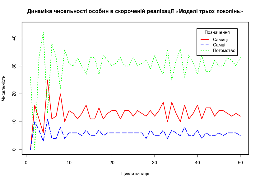

Fig. 8.3. The graph produced by R-script 8.2.
Could such a model have been constructed in LO Calc in a similar way? It could be constructed, but it would not function properly regardless... For example, we could fill only those cells of the spreadsheet that are necessary for building the output graph. All other quantities could be computed in cells that are recalculated with each "tick" of the counter. Unfortunately, this solution has a significant drawback: such constructs in spreadsheets operate with a large number of errors. A non-trivial property of LO Calc is that when scrolling the counter it sometimes does not update the values of cells not displayed on screen. Excel is no better — even models that operate entirely stably in LO Calc become overwhelmed in it. What is to be done? Use R!
8.3. The "Competitive Reduction Model"
As you will recall, at the end of Chapter 5 the construction of the "Competitive Reduction Model" was described. Although it retained a simplified description of population structure and the mechanism of offspring formation, it employed a mechanism for simulating competitive reduction that may, in the author's view, be used in quite serious models. Let us also build this model in R, and in doing so make use of yet another important advantage of R over LO Calc — vectorisation.
The basic structural unit in LO Calc and other spreadsheets is a cell — an individual variable that can be linked to other variables by certain relationships. This is optimal for building simple models, but leads to "sheets" of formulas and numbers when more complex models are involved. In contrast, the basic unit in the R language is a vector — a sequence of objects of a certain type. Individual objects in R are also defined as vectors. As a consequence, in R, unlike many other programming languages, operations on vectors are common and follow the same rules and command structure as operations on individual numbers. This property of R is called vectorisation. We will now apply it — and you will see that it allows the code to be radically reduced and simplified (R-script 8.3).
R-script 8.3. The "Competitive Reduction Model" with resource limitation in vectorised form

V <- 400 # Resource limit
p_f <- 0.6 # Proportion of females in offspring
t <- 50 # Number of simulation cycles
Groups <- c("f1", "f2", "f3", "m1", "m2", "m3") # Vector of group designations
AlphaNumber <- c(5, 3, 1, 5, 3, 1) # Vector of group abundances
Breed <- c(0, 2, 3, 0, 0, 0) # Vector of female fecundity values
Fertilizat <- c(0, 0, 0, 0, 1.5, 2) # Vector of male fertilisation capacity values
Surviv <- c(0.9, 0.8, 0.7, 0.7, 0.6, 0.5) # Vector of survival values
Compet <- c(0.6, 0.7, 0.8, 0.7, 0.8, 0.9) # Vector of competitive ability values
Demand <- c(4, 7, 10, 4, 6, 9) # Vector of resource demand values
Competitions <- matrix(NA, nrow = t, ncol = length(Groups)) # Table for results to be stored
colnames(Competitions) <- Groups # Column names are group designations
for (i in 1:t){ # Main loop
BetaNumber <- floor(AlphaNumber * Surviv + runif(1, min = 0, max = 1)) # Beta-abundances
GammaNumber <- BetaNumber * Compet # Gamma-abundances (quota-adjusted)
BetaDemand <- BetaNumber * Demand # Beta-demands (unreduced)
GammaDemand <- GammaNumber * Demand # Gamma-demands (quota-adjusted)
Way <- ifelse(sum(BetaDemand) <= V, 1, ifelse(sum(GammaDemand) >= V, 2, 3)) # Selection of reduction scenario
DeltaNumber <- switch(Way, # Reduction depending on scenario
BetaNumber,
floor(GammaNumber *V / sum(GammaDemand) + runif(1, min = 0, max = 1)),
floor(BetaNumber-(BetaNumber-GammaNumber) * (sum(BetaDemand) - V) / (sum(BetaDemand) - sum(GammaDemand)) + runif(1, min = 0, max = 1)) )
Competitions[i, ] <- DeltaNumber # Filling the corresponding row in the results file
ifelse (sum(DeltaNumber[Breed>0]) <= sum(DeltaNumber * Fertilizat), # Which sex determines brood number: females or males?
om_O <- floor(sum(DeltaNumber * Breed) + runif(1, min = 0, max = 1)), # Two variants for determining offspring number
om_O <- floor(sum(DeltaNumber * Breed * sum(DeltaNumber * Fertilizat) / sum(DeltaNumber[Breed>0]) ) + runif(1, min = 0, max = 1)) )
om_O_f0 <- floor(om_O * p_f + runif(1, min = 0, max = 1)) # Number of new females...
om_O_m0 <- om_O - om_O_f0 # ...and new males
AlphaNumber <- c(om_O_f0, DeltaNumber[1], DeltaNumber[2], om_O_m0, DeltaNumber[4], DeltaNumber[5]) # Transition to the next age
} # End of main loop
par(lwd=2, cex=0.9, font.lab=1) # Graphics parameters: line width, font size, font type
plot(Competitions[, "f1"], type="l", lty=3, col="#e699ff", # First line, age-I females
main="Vectorised implementation of the Competitive Reduction Model", # Title
xlab="Simulation cycles", ylab="Abundance") # Axis labels
lines(Competitions[, "f2"], type="l", lty=2, col="#ff00e6") # Second line, age-II females
lines(Competitions[, "f3"], type="l", lty=1, col="#ff0000") # Third line, age-III females
lines(Competitions[, "m1"], type="l", lty=3, col="#99e6ff") # Fourth line, age-I males
lines(Competitions[, "m2"], type="l", lty=2, col="#00e6ff") # Fifth line, age-II males
lines(Competitions[, "m3"], type="l", lty=1, col="#0000ff") # Sixth line, age-III males
legend("topleft", inset=.05, title="Legend", c("Females I", "Females II", "Females III", "Males I", "Males II", "Males III"),
lty=c(3, 2, 1, 3, 2, 1), col=c("#e699ff", "#ff00e6", "#ff0000", "#99e6ff", "#00e6ff", "#0000ff" ))

Once the model has lost its non-deterministic character, one can calmly examine which values are obtained at which step, compare the computations with the original intention, and ultimately find the error. But how does one learn the intermediate values if R does not store them? By using special commands to force it to display all necessary steps in the console! To this end, the required print(VALUE) commands can be inserted into the script text, which will output the results of intermediate computations to the console. To understand what is what, print('TEXT') commands can also be inserted, which will output the necessary explanations.