Creation of Worlds — 09. Models Based on Cellular Automata

9. Cellular automata–based models
9.1. John Conway’s “Game of Life”
The “Game of Life”, created by John Conway, became a variant implementation of the ideas of two cybernetics classics: Alan Turing and John von Neumann. To understand the significance of this game, one must go through the main milestones of its prehistory.
The Turing machine, proposed in 1936, is an abstract executor that implements a certain algorithm by transitioning from one state to another. Turing’s idea was that a device capable of being in a finite number of states and executing certain algorithms could provide all sequences of actions used by humanity.
Von Neumann attempted to realize Turing’s algorithmic machine idea using a cellular automaton. A cellular automaton is a regular structure of cells, each of which can be in one of a finite number of states. To operate a cellular automaton one must set its initial state and the rules for cell transitions from one state to another. By the way, LO Calc and other spreadsheets are examples of cellular automata.
The von Neumann machine is a Turing machine capable of reproducing itself. In 1950 von Neumann succeeded in implementing this machine on a space of 200 000 cells, each of which could be in 29 states. The transition rules for each cell depended on the states of four neighboring cells. After creating the first von Neumann machine, much simpler implementations (requiring fewer cells and fewer states) were produced. To some extent, simplifying the von Neumann machine became one of the intellectual exercises for cyberneticians. The work described here was created in the course of this development. It, of course, does not implement a von Neumann machine, but it is a way to study properties of cellular automata governed by simple rules.
Mathematician John Conway published in 1970 in Scientific American (in the “Mathematical Games” column edited by the well‑known popularizer Martin Gardner) a description of the “Game of Life”. Its rules are extraordinarily simple (and this, in particular, determines its appeal).
The game is realized on a plane consisting of square cells. Each cell has eight neighbors (including those it touches at corners). Each cell can be in two states: “alive” (occupied, usually shown in black) and “dead” (empty, white). To start the game one must create an initial configuration (“first generation”).
Each subsequent generation is determined from the previous one according to two rules:
– a “dead” cell with exactly three “alive” neighbors becomes “alive”;
– an “alive” cell with fewer than two or more than three “alive” neighbors becomes “dead”.
Computing further generations makes sense while “alive” cells remain on the board or until the system enters a cycle, repeating one of its previous states.
These rules are sufficient to generate countless patterns (figures) that exhibit complex behavior. Many cell constructions quickly degenerate. Some turn out to be stable (for example, a block of four adjacent cells). There exist “gliders” – patterns that can cyclically change their configuration while moving indefinitely across the plane.
Initially Conway assumed that a pattern capable of providing unlimited continuation of the game and infinite increase of the number of alive cells (naturally, when using an infinite plane for the game) was impossible. Conway could not prove this statement and offered a prize for its proof or refutation. The prize was claimed by a group of hackers led by Bill Gosper: they spent a year and a half trying to create a pattern that would reproduce itself while generating other figures. In the jargon used to describe the Game of Life, this is called building a “gun” that shoots “gliders”.
The “Gosper glider gun” became the first pattern capable of existing indefinitely and producing an unlimited number of “alive” cells.
Of course, there is no special need to implement the Game of Life with LO Calc: many good implementations exist. For example, on this website one can both test any initial configuration and view numerous figures that have their own names, including the “Gosper gun”. However, since cellular automata created with LO Calc can be useful for solving biological problems, we will discuss the principles of building such models using the Game of Life as an example (Fig. 9.1).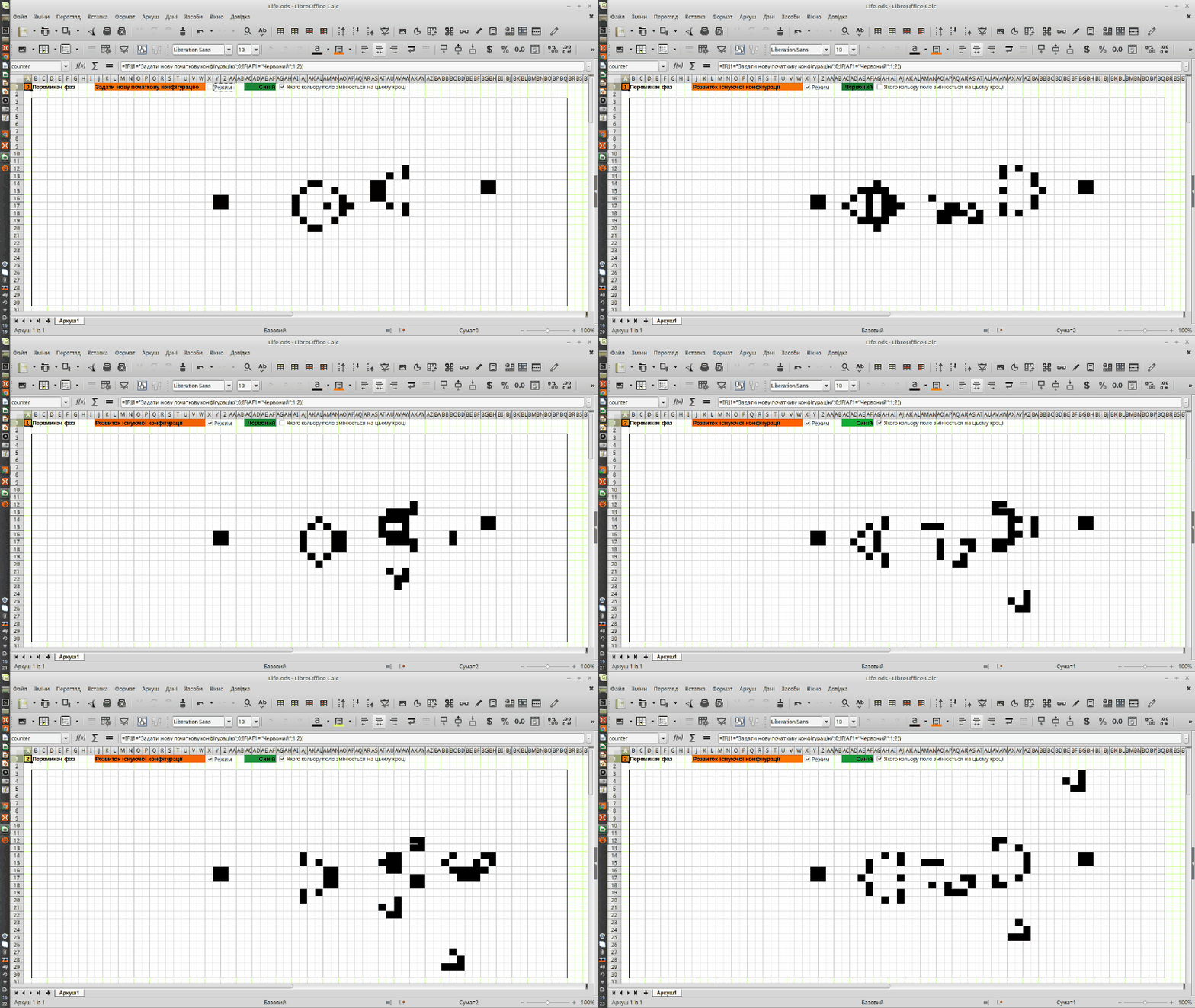

Fig. 9.1. “Gosper glider gun” in Conway’s Game of Life implemented in LO Calc (animated gif that starts moving after full loading)

9.2. Implementation of the Game of Life in LO Calc
Consider an example of the Game of Life implemented in LO Calc. It can be downloaded, but it is better to create it yourself.
Obviously, the Game of Life can be realized in LO Calc in many different ways. Most software solutions for this game use a single field. The cells of this field first store the initial configuration and then rebuild it step by step. These same cells show their state to the user by changing colour.
We will implement a different variant: we will build four separate fields. The first will be a “display” that reflects the game state; the second will be used to record the initial configuration; the third and fourth will sequentially provide the reconstruction of the pattern generated by the game (Fig. 9.2). In addition to greatly simplifying the formulas that have to be used, this solution makes analysis of why the model behaves in a particular way easier. At each stage one can look at the initial configuration reflected on the yellow field and compare two consecutive steps of the model (on the blue and red fields, or vice‑versa on the red and blue fields).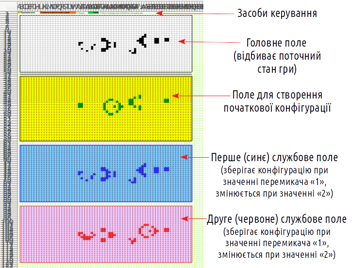

Fig. 9.2. Model from “bird’s‑eye view”. Shows the use of four different fields that share the same configuration and refer to each other
First of all, the model can operate in two modes: setting the initial configuration and developing the existing configuration. Switching between these modes is provided by a switch located in cell X1 (Fig. 9.3). The “Switch” control in the “Form Controls” menu has slightly different functions; in the discussed model a “Check Box” is used, where one can tick or untick to switch between the two modes. Depending on the state of this switch (we will keep calling it that) the label on the red‑background cell changes to indicate the active mode.
Puzzle 1. How is it arranged that, depending on the switch value, the value of the cell on the red background (J1) changes? This cell is controlled by the “Check Box” placed in X1.
In the development mode the existing configuration must be rebuilt step by step: first the red field is rebuilt based on the blue one, then the blue field based on the red one. For this a second “Check Box” – a field switch – is used. It controls cell AF1. Thus the model can be in one of three states: setting the teaching configuration, rebuilding the red field, or rebuilding the blue field. The choice of the current state is made by a phase counter located in cell A1. The formula assigned to it is simple: =IF(J1="Set new initial configuration";0;IF(AF1="Red";1;2)). You understand that double quotes mark the textual values of cells referenced?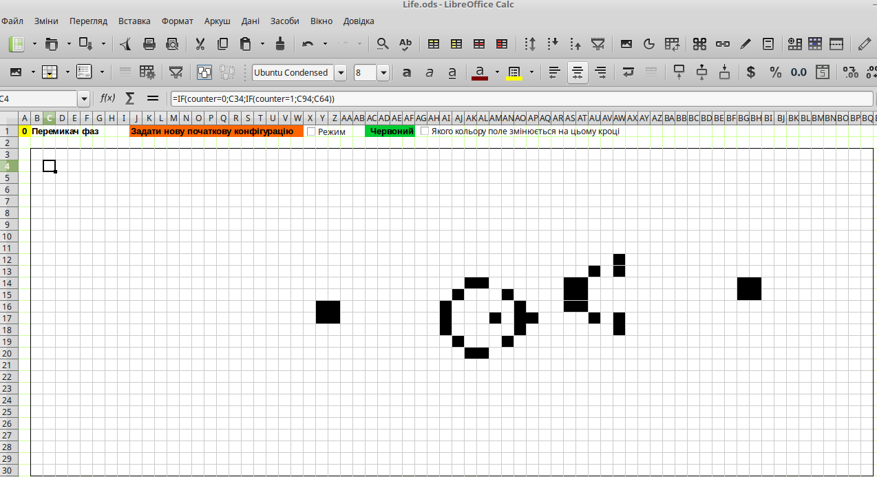

Fig. 9.3. The white field is the main one; it reflects the current state of the game
The cells of the white field reflect the state of the yellow‑field cells when the phase counter is 0, the state of the red‑field cells when the counter is 1, and the state of the blue‑field cells when the counter is 2. For example, for cell B3 the formula is: =IF(counter=0;B33;IF(counter=1;B93;B63)).
Puzzle 2. How is it arranged that the cells of the white field B3:BQ30 (Fig. 9.3) are purely white when the value is 0 and purely black when the value is 1?
Working with the yellow field is straightforward. Its cell values must be changed manually, using 0 and 1 or vice‑versa. Conditional formatting paints zeros yellow and ones green (Fig. 9.4).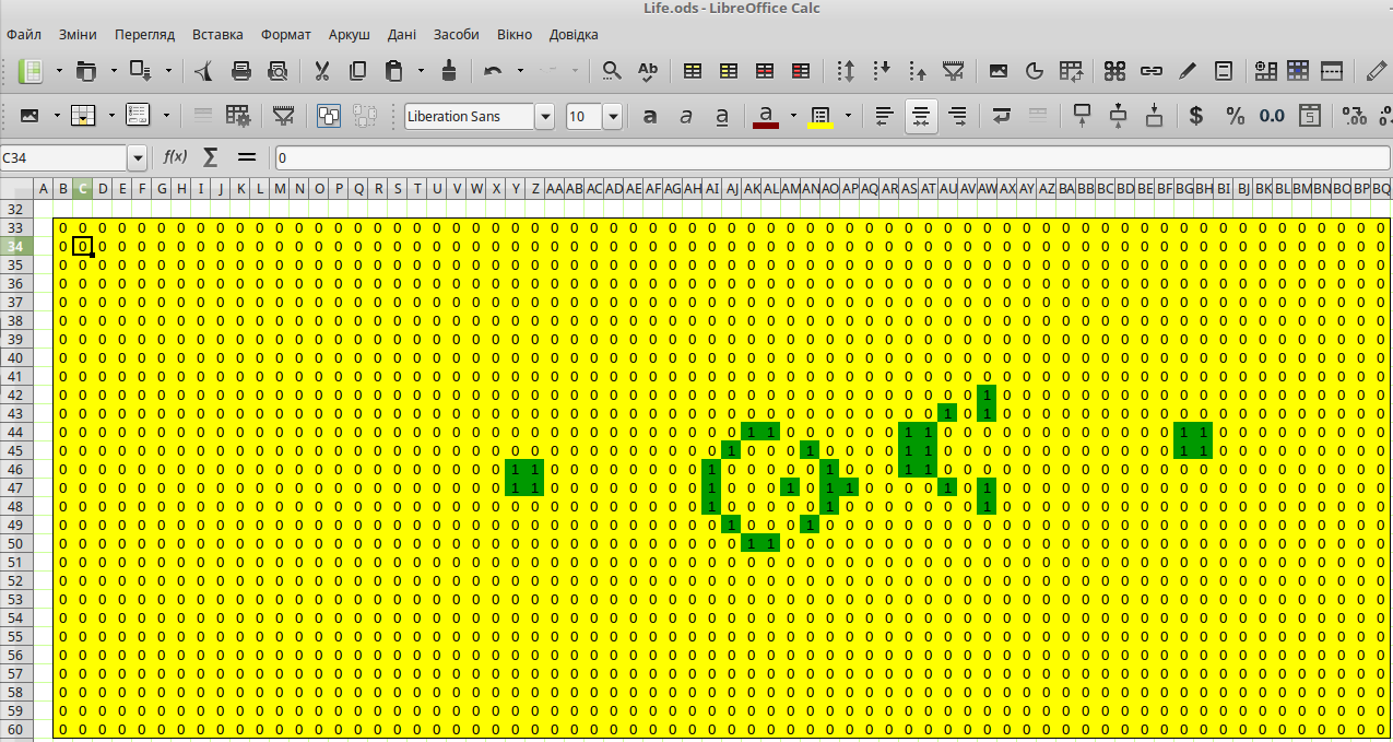

Fig. 9.4. On the yellow field one can set the initial configuration (the phase switch must be in state 0)
The blue and red fields are “twins” – each, in development mode, is rebuilt in turn based on the pattern on the other field. Consider the formula in cell C64 shown in Fig. 9.5:
=IF(counter=0;C34;IF(counter=1;C64;IF(counter=2;IF(C94=0;IF((B93+C93+D93+D94+D95+C95+B95+B94)=3;1;0);
IF((B93+C93+D93+D94+D95+C95+B95+B94)>3;0;IF((B93+C93+D93+D94+D95+C95+B95+B94)<2;0;1)));C94))
To understand this formula, note that the “reflection” of cell C64 (on the blue field) is cell C94 (on the red field). Cells B93, C93, D93, D94, D95, C95, B95 and B94 are its neighbors. As you recall, a cell remains “alive” only if it has exactly three “alive” neighbors.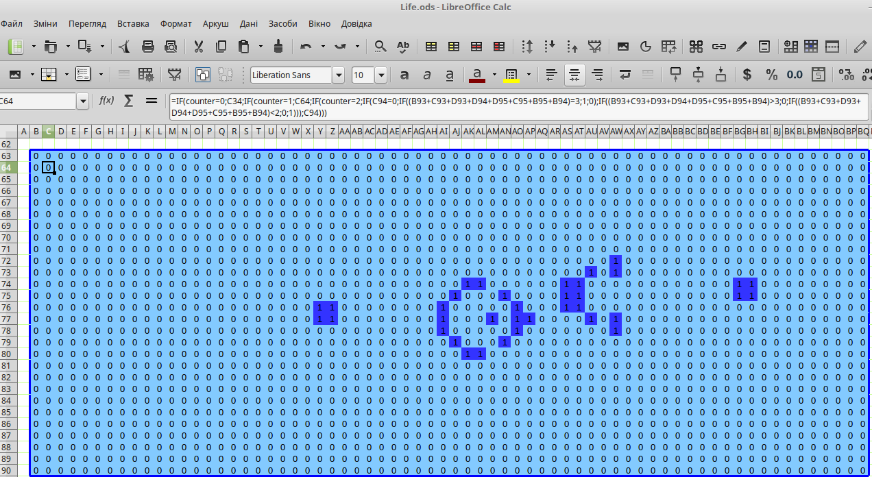

Fig. 9.5. The blue field is rebuilt when the phase switch has value 2
Cell B63 has a slightly different formula:
=IF(counter=0;B33;IF(counter=1;B63;IF(counter=2;IF(B93=0;IF((BQ120+B120+C120+C93+C94+B94+BQ94+BQ93)=3;1;0);
IF((BQ120+B120+C120+C93+C94+B94+BQ94+BQ93)>3;0;IF((BQ120+B120+C120+C93+C94+B94+BQ94+BQ93)<2;0;1)));B93))
This is related to the fact that the Game of Life board is infinite. Cell B93, located in a corner, borders cell BQ120 in the opposite corner, as well as BQ93 on the opposite horizontal side and B120 on the opposite vertical side – verify this yourself using Fig. 9.6!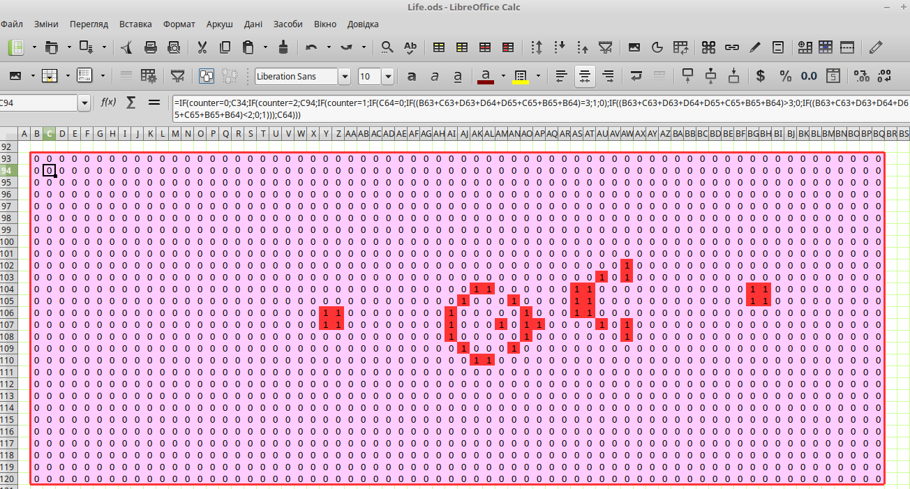

Fig. 9.6. The red field is rebuilt when the phase switch has value 1
Thus, using the model is uncomplicated. Switch the mode to set a new configuration; switch again and start “clicking” the switch that selects the fields to be updated. Observe the changes in “Life” step by step…
…and don’t forget to find the answers to the puzzles!