Creation of Worlds — 10. Examples of various models, their concept and design

10. Examples of various models, their concept and design
10.1. A selection of models for familiarization with construction options
It is undeniable that in order to successfully use simulation modeling in one’s work, a biologist must be able not only to use the simplest tools for building models. He must see situations in which modeling can help him, be able to formulate the task that the model should solve, and also develop the model design—a set of input parameters, computed quantities, relationships among them, and, ultimately, a set of output parameters of the model.
How to learn this? By analyzing others’ models and creating one’s own.
The author of this course suggests examining several models that he has had to develop to solve various tasks. These models are far from being exemplary (rather the opposite); however, students can gain useful experience not only by analyzing the merits of existing models but also by considering their shortcomings. The models whose examples are given here were created to illustrate certain points discussed in the columns (articles reflecting the author’s view) in the journal “Kompyuterrra”. To understand the structure and features of the models, one must read the columns themselves (and, if necessary, the sources cited by those columns) and see where the examined models are “embedded”.
47. When does selection become ineffective? The model from this column can be downloaded here.
50. Altruism and Simpson’s paradox. The (bulky, “ugly”) model from this column can be downloaded here.
51. Supports of altruism. The model from this column is placed here.
137. Discussion of the transition from hermaphroditism to separate sexes as an example of non‑classical development of a natural‑science hypothesis. The model for this column is described below and is available in a version for Excel‑2013 and in a version for Excel‑2003.
138. On the nature of male and female, or from conjugation to oogamy. Here are the model variants for Excel‑2013 and for Excel‑2003.
The boys‑and‑girls problem. This problem sparked controversy. The simplest way to obtain an unambiguous answer is to build a model.

— provide the possibility for each group of individuals to set its preferences regarding pair formation with representatives of all other groups;   — provide, among possible states of the "sex" trait, variants of hermaphroditism and parthenogenetic females (including those that require mating with some male for reproduction); this is connected with the fact that the model being created should be suitable for modeling the evolution of separate sexes, described in the series of "sex" columns: first, second, third, fourth, fifth, sixth, seventh, eighth, and the final one;	— provide the possibility to set the dynamics of carrying capacity (stochastic; in accordance with some cycle; cyclic with a stochastic component);	— provide the possibility of switching ontogenetic strategies depending on the competitiveness level of the environment.
The last requirement imposes serious limitations on the method of model implementation. Both in the Batrachometrics model and in Anton Leonov's model, not individual organisms but groups consisting of identical individuals (belonging to the same form and having the same age) were considered as separate units. In the Gause-100 model, individual organisms are considered as separate units (although individuals of the same form and age remain identical). In the Gause model, individual organisms should be considered as separate units, and moreover, each organism's characterization should include a number of its traits, first and foremost — the nature of its ontogenetic strategy. This means that the model must include a mechanism for determining these strategies and managing them.
10.5.2. Ontogenetic Strategies of Individuals
An important reason for creating the Gause model is the modeling of ontogenetic strategies. First of all, it is necessary to understand what they represent. Currently, species strategies (primarily r- and K-) are best described. The concept of strategy remains confused. In the most general form, a strategy can be defined as a hierarchy of priorities (more detail — here). The most common representations of strategies are as different variants of choice between the organism maintaining itself and reproducing itself in offspring. The diversity of green frogs and many other animals in their growth rate, age at first reproduction, fecundity, and life duration can be described as manifestations of ontogenetic strategies. The concept of ontogenetic strategies is introduced in this article; there descriptions of dwarfism and early maturation strategies are also given. In accordance with the initial assumptions, we expected that two alternative strategies could be described as follows.
Strategies

10.2. Epidemic dynamics model
Below is a description of how to create a simple model that describes the spread of an epidemic. This model can be downloaded from the site or built independently according to the description (the latter is preferable).
The model considers four individual states: susceptible (code 1), sick (2), immune (3), dead (4). For modeling, transition probabilities between these states must be set: infection of a susceptible when a sick individual is nearby (1→2), and recovery of a sick individual and its transition to the immune state (2→3). The probability of death of a sick individual is one minus the probability of its recovery.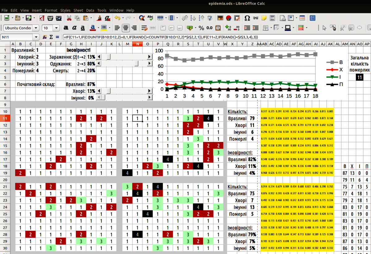

Fig. 10.1.1. Epidemia model window
To control changes of these teaching parameters you can use a scroll bar. To insert a scroll bar, go to “View / Toolbars” and select the “Form Controls” toolbar. This toolbar will appear on the LO Calc sheet. Switch to design mode using the button labeled “OK”: “Design Mode”. Control elements will become available, among which you can choose a scroll bar. After selecting it, draw a rectangle on the sheet; LO Calc will insert the control there. Depending on the shape you draw, the scroll bar will be horizontal or vertical.
To configure the scroll bar, select it while remaining in design mode. The “Control” button with crossed tools becomes active. Clicking it opens the dialog “Properties: Scroll Bar”. On the first tab, “General”, you can set properties such as size, position, minimum and maximum values, step size, etc. On the second tab, “Data”, you must specify the cell whose value will be changed by the scroll bar. After the control properties are set, you can simply close the dialog: the changes will be saved. Note: the scroll bar will work only after you exit design mode! To change its position or other properties you will need to re‑enter design mode.
One way to use the scroll bar is as follows. The bar controls the value in a particular cell (which may be hidden under the bar itself). This cell’s value ranges from 1 to 100. In the cell where the initial parameter value is calculated, a formula divides the scroll‑controlled cell value by 100. This value can be displayed as a percentage. This more complicated route is needed because the scroll bar can only set integer values, while the initial parameters (probabilities) must be expressed as fractions of one.
In addition, the number of initial parameters includes the initial population composition. This can also be set with scroll bars. For example, you can define the proportion of sick individuals and the proportion of immune individuals; all remaining individuals are susceptible.
The simplest way to build the model is as follows. On a certain area (in the example this is a 10 × 10 rectangle, but any other layout is possible) randomly place individuals according to the distribution defined by the initial parameters. For each cell on this field you must determine which individual occupies it. For such tasks you compare a random number (from 0 to 1) with the distribution of a unit. If we dealt with two cell states (e.g., white and black), we could generate the random number directly in the formula (if the random number is less than the probability of a white cell, the cell is white; otherwise it is black). We use a distribution with three states; in a single formula the same random number cannot be simultaneously compared with two different thresholds. Therefore, somewhere on the Calc sheet a field of random numbers must be placed (in the demonstration model this field is highlighted in yellow). Each cell of this field contains the formula =RAND().
Now, in the initial distribution field you can determine which individuals occupy each cell. This is done with the formula =IF(random_number<$susceptible_share;1;IF(random_number<($susceptible_share+$sick_share);2;3)). Each cell of the initial‑value field refers to its own random number; the shares of susceptible and sick individuals, set by the initial parameters, are the same for all cells in this field. The formula first compares the random number with the susceptible share (probability). If it is lower, a susceptible individual appears in the cell. If the random number exceeds that probability, it is compared with the sum of the probabilities of susceptible and sick individuals. If lower, the individual will be sick; if higher, immune. Such formulas allow the required area to be filled with randomly placed individuals whose appearance probabilities are defined by the initial parameters.
The initial distribution must then change. Susceptible individuals adjacent to sick ones may become infected. Sick individuals may recover or die. To show these changes we need another field (another rectangle of the same size as the initial distribution rectangle and the random‑number rectangle). Each cell here contains a fairly complex formula.
=IF(initial_cell=1;IF(COUNTIF(neighbor_cells;2)=0;1;IF(RAND()<COUNTIF(neighbor_cells;2)*$infection_prob;2;1));IF(initial_cell=2;IF(RAND()<$recovery_prob;3;4);3)).
To determine how many sick individuals border a susceptible one, select a 3 × 3 block and count the number of sick (twos). Thus, if we want to know how many twos border cell C11, we can use COUNTIF(B10:D12;2). Cell C11 itself is also included in this block, but this does not affect the calculation because it contains a one, not a two. The infection probability is the product of the number of sick neighbours and the probability of catching the disease from a sick neighbour. To decide whether a particular individual becomes sick, the random number is compared with this product; if the random number is less than the product, the individual becomes sick. Note that the product can exceed one (e.g., a susceptible individual has three sick neighbours, each with infection probability 0.5, giving a total > 1); in that case the random number will always be less than the product and the individual becomes sick with probability 1.
If the cell of interest contains a sick individual, it may recover or die. In this case its fate is also determined by comparing a random number with the probabilities given in the initial parameters. If the initial‑distribution cell contained neither a susceptible nor a sick individual, it contained an immune individual, which will remain immune.
Now you can count how many of each type of individual are present in the updated distribution. Use formulas such as =COUNTIF(range;1). “range” is the field with the updated distribution. This formula counts susceptibles; similarly, =COUNTIF(range;2) counts sick individuals.
Based on the numbers of susceptibles, sick and immune individuals, calculate the probabilities of each type appearing in the next distribution. Suppose that where dead individuals were, new individuals will appear (with characteristic probabilities). Then the probability of susceptibles in the next step is =num_susceptible/(num_susceptible+num_sick+num_immune).
Now build the initial distribution for the second cycle of the model. It is constructed in the same way as the first initial distribution, but using the probabilities calculated after the first cycle instead of the original ones. Naturally, a new field of random numbers will be needed. One can also experiment with a variant where the second‑cycle distribution is generated by the random‑number field of the first cycle.
To build the updated distribution for the second cycle you can copy the appropriate cells from the first cycle.
Before copying the second cycle to the third, remove absolute references ($) from the formulas. If you do not, the initial field of the third cycle will be built according to the probabilities calculated at the end of the first cycle, not the second.
To make the distributions visually assessable at a glance, use conditional formatting. Highlight the original and updated distributions. Go through “Format / Conditional Formatting / Condition”. For each possible value choose a style. The distribution becomes more illustrative…
To plot a graph, place the numbers of susceptibles, sick, immune and dead individuals for each cycle in one group. Stack these groups vertically and build a chart from the data.
10.3. Transition from hermaphroditism to separate sexes
Detailed description of the model illustrating the processes discussed in the column on the transition from hermaphroditism to separate sexes. The model is built in Excel‑2013. It can be downloaded via this link, and a version for Excel‑2003 via that link (the functionality of the second version has not been tested!).
The model consists of an Excel sheet containing a block for entering initial‑parameter values, a calculation block (based on difference equations), and a results‑display block (chart). The blocks are arranged so that everything needed for experimenting with the model fits on the initial screen.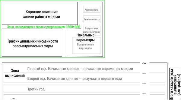

The appearance of the model’s initial screen is as follows.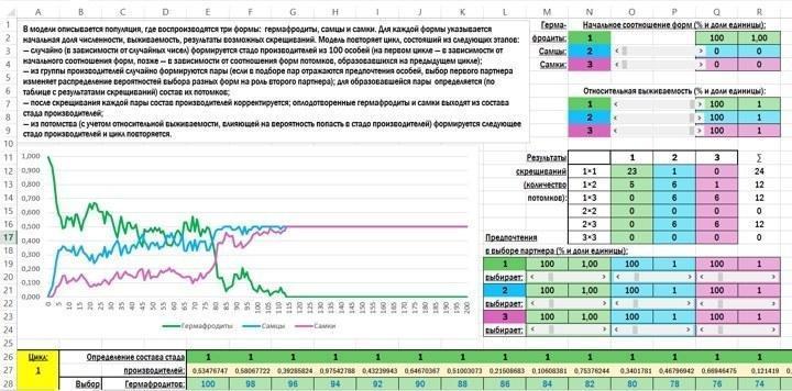

Below is the description of the model’s operation that is included in the file itself:
The model describes a population in which three forms reproduce: hermaphrodites, males and females. For each form the initial proportion, survival, and possible crossing outcomes are specified. The model repeats a cycle consisting of the following stages:
— randomly (according to random numbers) a herd of producers of 100 individuals is formed (in the first cycle according to the initial form ratios, later according to the offspring form ratios from the previous cycle);
— from the producer group random pairs are formed (if pair‑selection preferences are reflected, the choice of the first partner changes the probability distribution for the second partner’s form); for each pair the offspring composition is determined (by a crossing‑result table);
— after each pair’s crossing, the producer composition is updated; fertilized hermaphrodites and females leave the producer herd;
— from the offspring (taking relative survival into account, which influences the chance of entering the producer herd) the next producer herd is formed and the cycle repeats.
In the block for setting initial parameters, control elements called scroll bars are used.
The model uses coding: hermaphrodites are denoted by 1, males by 2, females by 3. Cells that may contain these symbols are highlighted differently depending on which symbol they hold.
When the initial population size (initial form ratios) is set with scroll bars, the percentage share of males and females is set (range 0 %–50 %); the number of hermaphrodites is then determined.
When relative survival is set with scroll bars, survival for all three forms is set from 0 % to 100 %. Absolute survival is not considered in the model. For example, from 1000 hermaphrodites 8 survive, from 1000 males 10 survive, from 1000 females 5 survive. In this case the relative survival of males (the most successful sex) is 100 %, hermaphrodites 80 %, females 50 %.
In the crossing‑result table, at the intersection of rows and columns corresponding to the two partners, the number of offspring is indicated.
Partner‑choice preferences are set with scroll bars. All values range from 0 % to 500 %. A value of 100 % corresponds to equal probability; lower values reduce the probability, higher values increase it.
A fragment of the working area of the file with explanations of what is calculated in its cells is shown in the figure.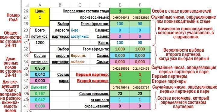

Initially the composition of the producer herd for the first year (calculation cycle) is placed in row 26. All 100 individuals are calculated at once. Subsequent calculations proceed down the columns within the row block corresponding to the year. The easiest way to describe the calculations used is to list these cells in order, using row addresses. Formulas copied from the model cells are highlighted in yellow.
F26 — =IF(F27<$R$2;1;IF(F27<($R$2+$R$3);2;3)) — formula determining the sex of an individual in the spawning herd, based on the random number in cell F27. $R$2 and $R$3 are the cells containing the proportions of the different sexes in the population. In later years the same calculation uses the sex ratios obtained from the previous year (A39, A40 and A41 for the second year).
F27 — =RAND() — a random number generated by the program, ranging from 0 to 1; used to determine the sex of one individual from the producer herd (cell F26).
F28 — =E28-(IF(E36=1,IF(E37=1,2,IF(E37=2,1,0)),0)+IF(E37=1,IF(E36=2,1,0),0)) — calculates the number of hermaphrodites in the producer herd that can participate in matings. It is based on the value in cell E28 (total hermaphrodites before pairing) and the sexes in cells E36 and E37, which recorded the sexes of the individuals forming the previous pair. If a hermaphrodite was paired with a male or another hermaphrodite, it became pregnant and left the producer herd.
F29 — =E29 — calculates the number of males in the producer herd that can participate in matings. This number is equal to their initial number in the producer herd, because males do not become pregnant and can mate repeatedly.
F30 — =E30-(IF(E36=3,IF(E37=1,1,IF(E37=2,1,0)),0)+IF(E37=3,IF(E36=1,1,IF(E36=2,1,0)),0)) — calculates the number of females in the producer herd that can participate in matings. Analogous to the hermaphrodite formula.
F31 — =SUM(F28:F30) — sum of the three previous cells.
F32 — =IF(F31<2,0,IF(F36=1,(F28-1)*$N$19/((F28-1)*$N$19+F29*$P$19+F30*$R$19),0)+IF(F36=2,F28*$N$21/(F28*$N$21+(F29-1)*$P$21+F30*$R$21),0)+IF(F36=3,F28*$N$23/(F28*$N$23+F29*$P$23+(F30-1)*$R$23),0)) — taking into account that cell F36 contains the first partner in the pair, this recalculates the probability that the second partner will be a hermaphrodite. $N$19 and other references point to cells where pairing preferences are set.If the total number of possible partners in the breeding stock is less than two, the value in the cell will be equal to 0.
F33 — =IF(F31<2;0;IF(F36=1;F29*$P$19/((F28-1)*$N$19+F29*$P$19+F30*$R$19);0)+IF(F36=2;(F29-1)*$P$21/(F28*$N$21+(F29-1)*$P$21+F30*$R$21);0)+IF(F36=3;F29*$P$23/(F28*$N$23+F29*$P$23+(F30-1)*$R$23);0)) — similar to the previous one; the probability that the second partner will be a male.
F34 — =IF(F31<2;0;IF(F36=1;F30*$R$19/((F28-1)*$N$19+F29*$P$19+F30*$R$19);0)+IF(F36=2;F30*$R$21/(F28*$N$21+(F29-1)*$P$21+F30*$R$21);0)+IF(F36=3;(F30-1)*$R$23/(F28*$N$23+F29*$P$23+(F30-1)*$R$23);0)) — similar to the two previous ones; the probability that the second partner will be a female.
F35 — =RAND() — a random number generated by the program, ranging from 0 to 1; used to determine the sex of the first partner in the pair.
F36 — =IF(F31=0;0;IF(F35<F28/F31;1;IF(F35<(F28+F29)/F31;2;3))) — the sex of the first partner in the pair, which is determined by the random number in the previous cell, depending on the number of potential partners in the breeding stock.
F37 — =IF((F32+F33+F34)=0;0;IF(F38<F32;1;IF(F38<(F32+F33);2;3))) — the sex of the second partner in the pair, which is determined taking into account the preferences for the first partner selection based on the values of the random number in the following cell.
F38 — =RAND() — a random number generated by the program, ranging from 0 to 1; used to determine the sex of the second partner in the pair.
F39 — =IF(F36=1;IF(F37=1;$O$12;IF(F37=2;$O$13;IF(F37=3;$O$14;0)));0)+IF(F36=2;IF(F37=1;$O$13;IF(F37=2;$O$15;IF(F37=3;$O$16;0)));0)+IF(F36=3;IF(F37=1;$O$14;IF(F37=2;$O$16;IF(F37=3;$O$17;0)));0) — the number of hermaphrodite offspring, determined depending on the pair composition.
F40 — =IF(F36=1;IF(F37=1;$P$12;IF(F37=2;$P$13;IF(F37=3;$P$14;0)));0)+IF(F36=2;IF(F37=1;$P$13;IF(F37=2;$P$15;IF(F37=3;$P$16;0)));0)+IF(F36=3;IF(F37=1;$P$14;IF(F37=2;$P$16;IF(F37=3;$P$17;0)));0) — the number of male offspring, determined depending on the pair composition.
F41 — =IF(F36=1;IF(F37=1;$Q$12;IF(F37=2;$Q$13;IF(F37=3;$Q$14;0)));0)+IF(F36=2;IF(F37=1;$Q$13;IF(F37=2;$Q$15;IF(F37=3;$Q$16;0)));0)+IF(F36=3;IF(F37=1;$Q$14;IF(F37=2;$Q$16;IF(F37=3;$Q$17;0)));0) — the number of female offspring, determined depending on the pair composition.
After the simulation of formation of 100 pairs has been performed, the overall results for the year are calculated. The cells where this is done are located in column A.
A31 — =SUM(E39:CZ41) — the total number of offspring produced in the given year (in the given cycle of the model operation).
A35 — =SUM(E39:CZ39)/A31 — the proportion of hermaphrodites produced in the given cycle of the model.
A36 — =SUM(E40:CZ40)/A31 — the proportion of males produced in the given cycle of the model.
A37 — =SUM(E41:CZ41)/A31 — the proportion of females produced in the given cycle of the model.
A39 — =A35*$R$7 — the proportion of hermaphrodites surviving to the next year (taking into account their survival rate set in the initial parameters).
A40 — =A36*$R$8 — the proportion of males surviving to the next year (taking into account their survival rate set in the initial parameters).
A41 — =A37*$R$9 — the proportion of females surviving to the next year (taking into account their survival rate set in the initial parameters).
The simulation results for each cycle of the model operation are displayed in the block of cells located in the rightmost part of the sheet. A graph, which is the main form of output of the model results, is constructed based on the set of numbers generated in this way.
Using the model is very simple. Using the block for determining the initial parameters, it is necessary to set a set of initial values. After that, all that remains is to press the F9 button, wait for some time, which is determined by the computer performance, and interpret the resulting graph.
10.4. Population Dynamics and Gause's Rule (at the Limits of Spreadsheet Capabilities!)
10.4.1. Model Gause-100
The author of this manual has created, using Microsoft Excel, a model describing the interaction of four competing forms, which may belong to one or different species. Unfortunately, independent accounting of a large number of individuals in a model population requires a fairly large amount of computation. The model presented here considers a guild (i.e., a set of forms using the same resource) consisting of 280 or fewer individuals, each of which belongs to one of four forms.
The model itself (named Gause-100) can be downloaded here. A detailed description will be given below. On one hand, this description will help during experiments with this model. It is equally important that this model should serve as a template for building a professional model written in Python. The description of the model made in Excel, as the author hopes, will help developers of its extended analogue in Python or another professional programming language.
The model serves for simulating population dynamics and competition of two competing species. It considers the interaction of four forms of organisms (females and males of the two species under consideration). Each form can be represented by individuals of four different ages (in total — 16 groups of individuals). Individuals belonging to one group (i.e., belonging to one form and having the same age) are considered identical.
The model allows changing several initial parameters characterizing each group of individuals, including setting the results of their mating. From the initial pool of individuals, the guild modeled by the model is formed (i.e., a set of individuals, including those of different species, that exploit the same resource). Competitive reduction of numbers is simulated in case the guild's resource needs exceed the carrying capacity of the environment. Then, pair formation (from among individuals capable of participating in reproduction, i.e., belonging to the breeding stock) and offspring production are simulated. In the next simulation step (in a typical case corresponding to a year), the new composition of the guild is formed from the previous one and the offspring that appeared in the previous step.
10.4.2. General Structure of the Model
The described model is constructed so that its input-output zone fits on a personal computer screen, allowing changes to the initial parameters and immediately observing the consequences of these changes.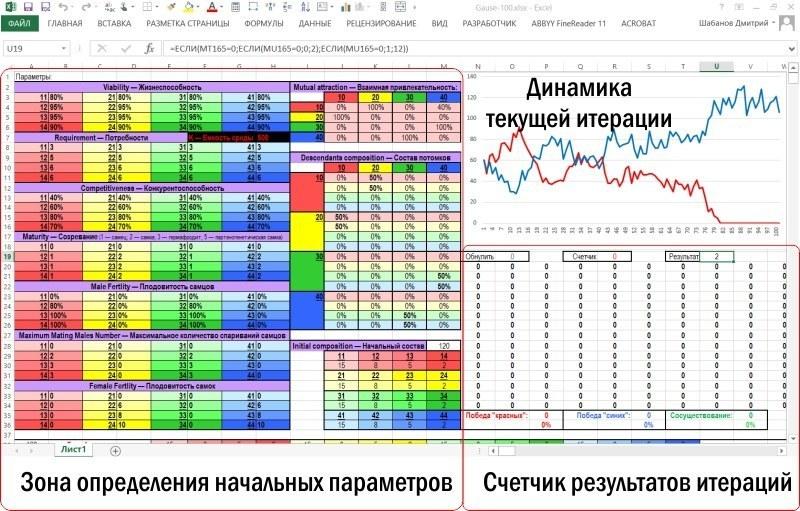

The model itself occupies a much larger space on the Excel sheet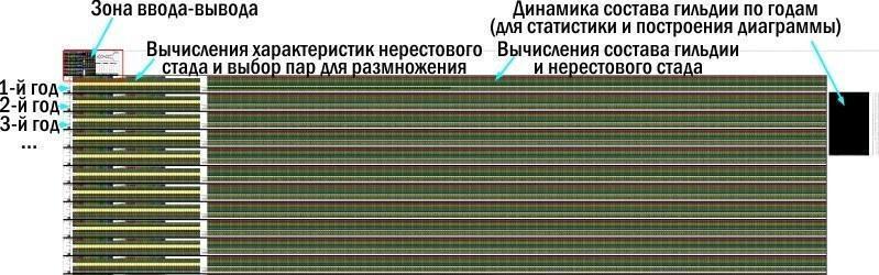

After the input-output zone, the computation zone is located. The computation zone for the characteristics of the breeding stock and pair selection for reproduction is larger than shown below. The figure shows a block of rows corresponding to the first year (a conditional year, of course, more precisely — the modeling step), and the beginning of the block corresponding to the second year.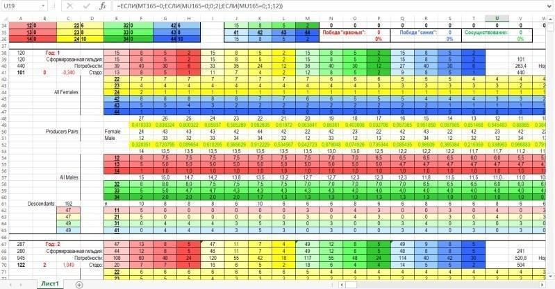

And the figure below shows the zone where the composition of the guild (the total set of individuals) and the breeding stock (the set of individuals participating in reproduction) is calculated.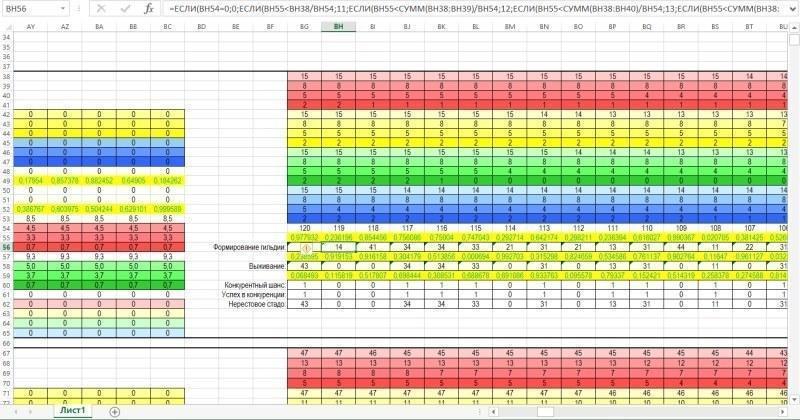

Finally, the next figure shows the zone where data on guild dynamics are collected based on the results of each year of modeling. Each row of this zone collects data from the corresponding rows of the computation zone. In the last two columns, the total number of representatives of the two species is calculated. These columns serve as the numerical material for constructing the diagram located in the input-output zone.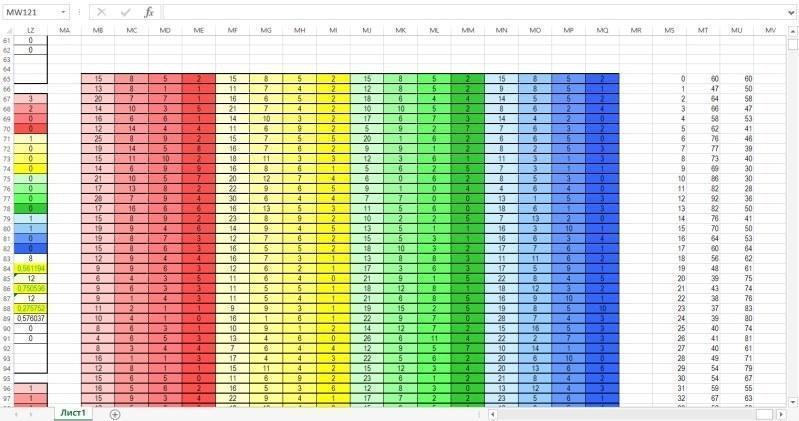

Viability parameters in the Gause-100 model:
— Viability;
— Requirement;
— Competitiveness;
— Maturity;
— Male Fertility;
— Maximum Mating Males Number;
— Female Fertility.
10.5. Requirements for the Professional Gause Model
10.5.1. General Characteristics
One of the main reasons for writing the planned model is that experiments with simpler models (initially the Excel model Batrachometrics-2010.xls, described here, and then — the professional model by Anton Leonov, briefly described here, and in more detail — in an article currently in press), revealed an effect, which we briefly reported in this publication. In our experiments, it was discovered when studying the patterns of competition between interspecific hemiclonal hybrids and individuals of one of the parent species. We assume that this is part of a broader pattern related to Gause's competitive exclusion principle. By the way, it is precisely with this that the name of the proposed model — "Gause" — is associated.
The task of the Gause model is simulation modeling of guilds (sets of populations, hemiclonal population systems, etc.), allowing study of the influence on their stability of competition, hybridization (including hemiclonal), diversity of ontogenetic strategies, diversity of reproduction methods, niche separation, and other similar population-biological phenomena.
In some important aspects, the work of the professional Gause model (probably written in Python) should resemble the work of the Gause-100 model. Nevertheless, the point of building a professional model is to obtain significantly broader possibilities for modeling as a result of its creation. In particular, this model should:
— simulate the dynamics of interaction not of four forms, but of a significantly larger number of them (for example, 22); this is connected with the fact that the same model should be suitable for modeling population systems of green frogs, including triploids (characteristic of the IV region of green frog distribution in the Left-bank Forest-Steppe of Ukraine), and for this it will be necessary to model a sufficiently large number of genotypes;
— provide the possibility for each group of individuals to set its preferences regarding pair formation with representatives of all other groups;
— provide, among possible states of the "sex" trait, variants of hermaphroditism and parthenogenetic females (including those that require mating with some male for reproduction); this is connected with the fact that the model being created should be suitable for modeling the evolution of separate sexes, described in the series of "sex" columns: first, second, third, fourth, fifth, sixth, seventh, eighth, and the final one;
— provide the possibility to set the dynamics of carrying capacity (stochastic; in accordance with some cycle; cyclic with a stochastic component);
— provide the possibility of switching ontogenetic strategies depending on the competitiveness level of the environment.
The last requirement imposes serious limitations on the method of model implementation. Both in the Batrachometrics model and in Anton Leonov's model, not individual organisms but groups consisting of identical individuals (belonging to the same form and having the same age) were considered as separate units. In the Gause-100 model, individual organisms are considered as separate units (although individuals of the same form and age remain identical). In the Gause model, individual organisms should be considered as separate units, and moreover, each organism's characterization should include a number of its traits, first and foremost — the nature of its ontogenetic strategy. This means that the model must include a mechanism for determining these strategies and managing them.
10.5.2. Ontogenetic Strategies of Individuals
An important reason for creating the Gause model is the modeling of ontogenetic strategies. First of all, it is necessary to understand what they represent. Currently, species strategies (primarily r- and K-) are best described. The concept of strategy remains confused. In the most general form, a strategy can be defined as a hierarchy of priorities (more detail — here). The most common representations of strategies are as different variants of choice between the organism maintaining itself and reproducing itself in offspring. The diversity of green frogs and many other animals in their growth rate, age at first reproduction, fecundity, and life duration can be described as manifestations of ontogenetic strategies. The concept of ontogenetic strategies is introduced in this article; there descriptions of dwarfism and early maturation strategies are also given. In accordance with the initial assumptions, we expected that two alternative strategies could be described as follows.

Dwarfism Early Maturation	Growth Rate (undersized)		Fecundity per Season (oversized)
	Coordinates	N	Coordinates	N
(undersized)	Large-sized lL = 9,7 + 8,3×A		Females bL = 32,5 + 8,3×A
The last requirement imposes serious limitations on the method of model implementation. Both in the Batrachometrics model and in Anton Leonov's model, not individual organisms but groups consisting of identical individuals (belonging to the same form and having the same age) were considered as separate units. In the Gause-100 model, individual organisms are considered as separate units (although individuals of the same form and age remain identical). In the Gause model, individual organisms should be considered as separate units, and moreover, each organism's characterization should include a number of its traits, first and foremost — the nature of its ontogenetic strategy. This means that the model must include a mechanism for determining these strategies and managing them. Males	Size lgme3 = 0,170; lgme4 =0,176		lL = 9.7 + 8.3×A bgme3 =0,450; bgme4 =0,288
bL = 32.5 + 8.3×A	Growth Rate at ages 3–4 years	Relatively low: lgme3 = 0.170; lgme4 = 0.176	Relatively low: lgme3 = 0.170; lgme4 = 0.176	Growth Rate Relatively early:
Strategies	Relatively late:		from 6 years
Relatively late:	Size F = ‑1325 + 335×A	‒	lL = 9.7 + 8.3×A F = 179 + 316×A	‒
Female Fecundity	Relatively low: F = -1325 + 335×A	— Relatively high:	F = 179 + 316×A —	Number of Reproduction Seasons Especially large:

Analysis of skeletochronological data obtained from the study of green frogs made it necessary to correct these concepts. Below is a table comparing two strategies of green frogs (the article from which it is taken is in press at the time of writing this page).

Age class
Characteristics

Especially small:
up to 3 years

Relatively small:
up to 4 yearsDescribing ontogenetic strategies, we calculate a Strategy parameter for each individual (depending on its size). It equals 1 if the individual’s size corresponds to the typical large‑size strategy, and ‑1 if it is typical of small size.
It is likely necessary to model individual differences by their ontogenetic strategies as follows. The Strategy parameter should become one of the characteristics of each individual. At present it is unknown how it is determined in reality. One may assume that this trait, like the overwhelming majority of other key individual characteristics, depends partly on the individual’s genotype and partly on environmental influences. The Gause model must provide for the possibility of simulating both mechanisms.

### 10.5.3. Modeling ontogenetic strategies
Based on an individual’s history, a characteristic value of the Strategy variable is determined. According to this value and the individual’s age, its viability, size, participation in spawning, and fecundity are determined. It is probably necessary to allow, for each of the 22 genotypes, two different variants corresponding to the extreme values of the Strategy parameter (for example, from +3 to ‑3). Naturally, the possibility of not specifying such variability must also be provided.
If the strategy is determined solely by belonging to a particular form, individuals with different strategies can be regarded as belonging to different forms, for which different parameter values are assigned.
If the strategy is determined only by the environment, for each form the extreme values must be set, and a function that adjusts the Strategy value at a certain age depending on a specific characteristic of the model guild (most likely competition intensity) must be provided.
The most difficult variant to implement is the one in which the strategy is partially determined by genetic predisposition and partially by environmental influence. I have no concrete solution to this problem at the moment of writing these lines. One possible approach is: include the state of several genes in each individual’s characteristics. The value of the Strategy parameter (and possibly other parameters, primarily those describing the efficiency of consuming different parts of the resource spectrum, as described in the next section) would be determined by rules that take these gene states into account. However, the implementation method for this variant still needs discussion.

### 10.5.4. Modeling niche partitioning
Since one of the tasks of the Gause program is to model competitive exclusion according to Gause, this model must include a mechanism for partitioning ecological niches. In this case, an ecological niche is the nature of the population’s relationship with its environment; niche partitioning is linked to the differentiation of resource niches, i.e., sets of consumed resources.
According to classical concepts, coexistence of competing species may be due to specialization on different parts of the shared resource spectrum. For example, species A and species B, existing alone, may consume the entire spectrum of available resources (e.g., feeding on both small and large prey, or feeding throughout the day). Gause’s rule states that if these two species live together, the stability of their coexistence can be ensured by them dividing resource niches: for instance, species A feeds on small prey while species B feeds on large prey, or species A feeds during the day and species B at night. Two or three variables by which niche division occurs (e.g., prey size, method of capture, and time of capture) allow stable coexistence of guilds consisting of a two‑digit number of populations.
I propose using a single parameter (prey size; however, it could be interpreted otherwise), consisting, for example, of 12 resource categories. The environment’s capacity (the amount of available resources) is set separately for these twelve categories (twelve numbers, not one as in the Gause‑100 model). Each form’s parameters include the efficiency of consuming each of these twelve categories.
A consequence of this algorithmic change is that the previous competitive reduction algorithm (which we were proud of) needs to be replaced or modified.
One variant is as follows. Each resource category is divided among all consumer groups (differing by form affiliation and age) that exploit it, proportionally to their abundance and their efficiency of consuming that category. The amount of resource obtained by each group is determined. Competitive reduction of individuals in that group then occurs, with each individual’s survival chance proportional to its competitive ability. In the simplest case, individuals of one group have equal competitive ability, but if individuals within the group differ in their ontogenetic strategies, their competitive abilities may differ.
A drawback of this algorithm is that, in the case of many competing groups, the probability of a sudden decline or increase in the size of any one group will be reduced. It is necessary to decide whether random deviation effects can be modeled when discretizing probabilities in small samples.

### 10.5.5. Interface features
Data entry into the model must be performed through five tables:
— viability parameter values for the considered individual forms;
— probability distributions for individuals of different forms (and ages?) choosing each other when forming pairs;
— probability distributions for offspring production from all possible mating combinations;
— initial guild composition and the predetermined pattern of immigration (arrival of certain individuals into the considered guild);
— composition and dynamics of environmental resources.

Designing the Gause model’s interface is a non‑trivial problem. Suppose the model considers 22 individual forms. The proposed number of individuals is not excessive. For example, the Batrachometrics model includes 13 forms: XLXL, XLYR, XRXR, XRYR, XR(XL), YR(XR), XR(YL), XL(XR), YL(XR), XL(YR), (XL)(XR), (XL)(YR), (YL)(XR). Anton Leonov’s model uses the same set of forms but remains open: new forms can be added (though currently in a user‑unfriendly way). An analysis of triploids would require adding a whole series of new forms. For each form, a lifespan must be specified. For green frogs, the maximum recorded lifespan is 10 years; when using the model for other forms, a substantially longer lifespan should be allowed. For example, gray toads, which we also use to study ontogenetic strategies, have a maximum lifespan of at least 15 years. Suppose we consider 22 forms (11 species if hybridization is absent) with a maximum lifespan of 16 years. This implies 352 age groups in the model. For each, a set of viability parameters must be defined. The Gause‑100 model uses 7 viability parameters. If the Gause model retains the same number of parameters (in reality their number should change, but not fundamentally), this means that assigning viability parameters requires filling 2 464 cells. The situation is aggravated by the fact that for at least some of these cells two values must be set: one for rapid maturation and one for slow maturation. Thus, the total number may exceed 5 000. To make entering such a volume of data feasible and meaningful, several mechanisms must be provided, including:
— automatic filling of cells according to a given template (the ability to create several templates of viability‑parameter values, then assign an appropriate template to each form, thereby automatically filling its cells);
— adjustment of automatically filled cells after applying a specific template;
— automatic disabling of unused cells (when the number of forms is less than 22 or the maximum lifespan is less than 16 years);
— export of completed viability tables to a simple format (e.g., *.csv) and their import.

An even more serious problem is determining the probabilities of individuals choosing each other when forming pairs. Under the assumed conditions, the model must consider 22 × 22 = 484 pairwise form combinations. However, this number may still be insufficient. In many cases, a crucial factor determining a partner’s potential attractiveness is its age (more precisely, age‑related parameters).

When determining offspring composition from matings, potentially 22 × 22 × 22 = 10 648 cells must be considered (for each pairwise mating of two forms, the probability of each of the 22 forms appearing in the offspring must be specified). Evidently, in the overwhelming majority of cases most of these cells will be unused. Most often, scenarios will involve only female and male forms; in this case only the cells corresponding to male‑female matings need to be filled. When modeling situations with hermaphrodites capable of hybridizing different forms, all cells will be needed; moreover, their number cannot even be halved, because offspring from a cross between two hermaphroditic forms A and B can differ depending on which parent performed the maternal role and which the paternal role.