SexOnR–02_R&other. R, RStudio, RMarkdown — first steps (R-handbook I)

02 R, RStudio, RMarkdown — First Steps
2.1 Some References
At the beginning of a course devoted to using the R language, it would be logical to include an overview of it. The author hopes to create such an overview in due course, building it in a way that emphasizes precisely those capabilities and features of the language that are important for the course. For now, this does not exist yet, and you will need to become acquainted with this language using other sources.
In Ukrainian, the following publication can be recommended (very successful, with very concentrated presentation):
Maiboroda R. Ye. Computer Statistics. K.: VPC «Kyiv University», 2019. – 589 p. This book will be our main one; fortunately, the author offers it for free distribution and use.
The author of this site began creating an overview of the R language in another course devoted to statistical analysis. This overview still needs to be refined and improved. Here are the materials that will be useful for this course.
Overview of the History of the R Language and Some Features of Working with It.
Statistical Oracle — 03. Using the R Language
Statistical Oracle — 04. Working with Data in R
Statistical Oracle — 07. Brief Overview of R Commands
Several more books, copies of which are located on this site, will also be useful; references to them are given in the aforementioned course.
How to Start Working with R? Download the R installer here and install it on your computer. After that, download RStudio and install it. Then you will open the RStudio window and interact with R through its assistance.
2.2 The RStudio Window
Launch RStudio. What will you see?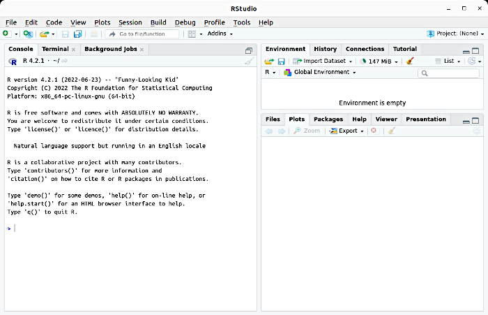

Fig. 2.2.1 We have just launched RStudio. This is what we see
The left part of the RStudio screen is occupied by the console — the «device» for input and output of information. After the > sign there is a cursor. Type 2*2 there and press Enter. You can see that you can use R in this mode, through the console.
In the right part of the RStudio screen you see two windows, each of which can be used differently depending on which tab is open there. At the top, the Environment window is currently open, where the objects that R will work with will appear. Below is the Plots window, where the graphs that the program will create will be displayed. Note that the borders between the windows are movable: you can «grab» them with the cursor and move them as needed.
However, we will not work with the console but with the script window. Open the RStudio menu and suggest creating a new file. You will see an additional menu where you will need to choose the type of such file.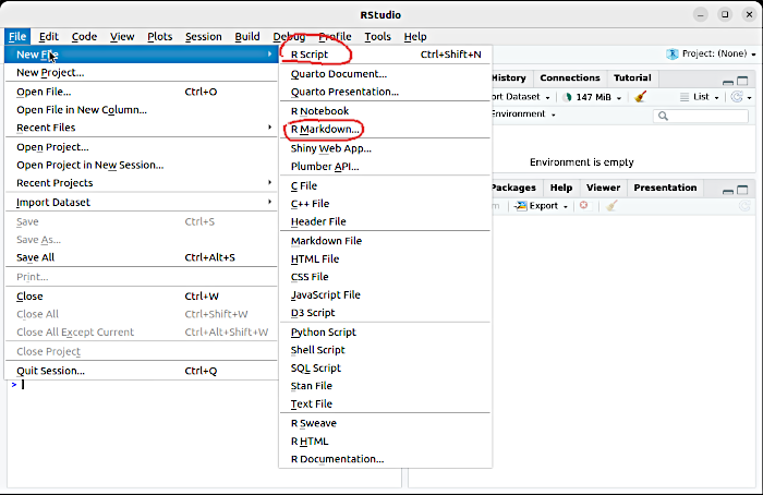

Fig. 2.2.2 This is how new windows for scripts and RMarkdown documents are opened
We will work with two types of files. First of all, these are R scripts (sequences of commands). Such files have the *.R extension. It is in them that we will write and save the models that we will create in this course. This is a much better solution than working in the console. In a script, you can gather a sufficiently large sequence of commands and add all necessary explanations to them. These commands can be run separately from others, or the entire sequence can be executed as a single whole. When working on improving a model, you can, for example, block a certain line from execution (for this, put a «hash», #, in front of it) and add some alternative command; run the script with this alternative and compare the results. A script can be made more understandable by using comments right in the lines where the commands are located; for this, it is sufficient to put a «hash», #, after the «working» part of the line, and then provide any explanations. Let's see how this works with a very simple example.
2.3 Executing a Trial Script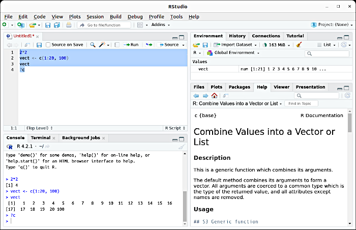

Fig. 2.3.1 The sequence of commands highlighted in the script window was executed by the Run button. The consequences of its execution are visible in all other windows of RStudio
A very simple (and actually meaningless) sequence of commands is written in the script window. The script lines are numbered. This script was selected entirely, and then the Run button located above this window was pressed; as a result, the result of sequential execution of the provided commands appeared in the console. The first of them is the arithmetic expression 2*2. In the console after the > sign, which demonstrates that the user can enter a command there, the command obtained from the script window was entered. Below is the system's response; it is located after the system message with the number of the provided element in the response line: [1]. Why is this number needed? This is useful when the response consists of several elements, as in the case of the command from line 3. But first, the command from line 2 should be executed.
Line 2 reads: vect <- c(1:20, 100). This command creates an object called vect (with this name we demonstrate that the basic type of objects in R are precisely vectors — ordered sequences). Creation occurs as follows: we name the new object and define it using the <- command. This assignment symbol is very characteristic of the R language; if you see it in a program, you will understand in which language it is written. To enter this command, it is sufficient to press Alt + dash (-) on the keyboard. Instead of these two symbols, one could also use =, and even (in cases where the definition precedes the object name) the symbols ->. Such commands will work, but... they are not widely used. The equals sign is used in other meanings, and when creating (or redefining already created!) objects, it is more convenient when the line begins with the object name.
What is the «content» of the new object? It is created by the function c(). The function name is an abbreviation either from the word concatenate or from the word combine, and it combines the arguments that are listed in the parentheses separated by commas. By the way, in R, a comma cannot be used as a decimal separator; 1,5 is not one and a half, but 1 and 5 (and this is one of the reasons why in such cases it is better to put a space after the comma). So, the function c() combines the result of executing the command 1:20 and the number 100. What is 1:20? It is a sequence of natural numbers from 1 to 20. An important feature of R (and not only of it) is that the same result can be obtained in many different ways. For example, the sequence from 1 to 20 can be obtained simply by listing it through the function c() — namely c(1, 2, 3, 4, 5, 6, 7, 8, 9, 10, 11, 12, 13, 14, 15, 16, 17, 18, 19, 20). The same can be obtained using the function seq(). In the parentheses of this function (its name, as one can easily guess, comes from sequence) its arguments are given. This function can also be used in different ways. Look at the list of R commands provided here; this command is in the section «7.5. Creating Objects». There it says the following:
seq(from, to, by = ) — generates a sequence of numbers from from to to with step by;
seq(from, to, len = ) — generates a sequence of numbers from from to to of length len.
Thus, the same sequence can be created by the commands seq(1, 20, by = 1) and seq(1, 20, len = 20). You understand that in both cases a different step of the arithmetic sequence than 1 can be set. By the way, in these commands we can see a different use of the = symbol than in the assignment procedure. And one more way (it is listed first in the section «7.5. Creating Objects») is simply using the command :. In the case shown on the screenshot, this simplest method was used.
After we created the object vect, RStudio showed in the console that it received this command (and if it received it and did not report an error — we understand that it executed it!). However, another important change occurred: as can be seen on the screenshot, this object appeared in the Environment window.
The next command of the script (line 3) names this object. RStudio in the console shows that it received this command and in response output this object to the console. Now we can understand why elements are numbered in square brackets. The first line contained 16 elements, and the second one begins with element No. 17.
Line 4 of the script remains. There the command ?c is given. This is a call for help regarding the command c. We see that in the lower right part of RStudio switched to the Help tab and offered an overview of the command we asked about.
A person who starts working with R most likely has a typical question. How to remember all these commands? When you advance further in working with this tool, you will be sure that the situation is not as terrible as it may seem at the beginning. The simplest commands you will remember quickly, because you will have to use them quite often. With more complex commands it is somewhat more complicated, but overall it is not tragic at all. It is important that you either remember that some problem can be solved using some function, or at least have hope for this. Then you need to find an example, understand how it works, and adapt it to your own needs. At first this seems complicated, but each time it becomes easier and easier. Over time, you will have scripts written by you and their drafts, where a collection of commands needed to solve your tasks will be gathered. The further you advance in mastering R, the easier it will be for you to take the next steps. By the way, the author of this text regularly forgets which commands should be used in one case or another. Remembering this, among other things, is helped by the R-wizard GPT-chat.
2.4 Creating an RMarkdown Document
RMarkdown is a text markup language embedded in RStudio. This is a tool that allows, using RStudio, to obtain a document that can be converted into many different formats, including *.pdf, *.html, *.docx, etc. Its main advantage is the ability to insert fragments of R-scripts and the results of their execution directly into the text.
In general, a fundamental feature of a scientific text is the focus not just on reporting conclusions, but also on explaining where they came from. In the case of simulation modeling, statistical analysis, this means special attention to the parameters of the models' operation, the data that were analyzed, and the features of the algorithms used. When it comes to a scientific article reporting the results of using R, it is often necessary to find a non-trivial compromise between the completeness of the text and the possibility of its perception. Sometimes it is necessary to report the main conclusions in the «body» of the article, and place the R-script text with comments in the appendices. In the same case, when it comes to educational texts, reports, qualification works, quite often the optimal solution is to combine R-code and sufficiently detailed comments. The best solution for this is RMarkdown. By the way, RMarkdown may be useful even for the person who writes the R-script themselves, builds the R-model. Time will pass, and you will forget why you did one thing or another. If you leave a written RMarkdown report, you will not only be able to explain your logic to someone else; you will make it understandable for yourself in the future!
Fig. 2.2.2 shows how to open a new RMarkdown document. It will be saved with the *.Rmd extension.
By the way, when working on a computer with a sufficiently wide screen, the author of this text likes to open a separate column in RStudio for RMarkdown documents (Fig. 2.4.1).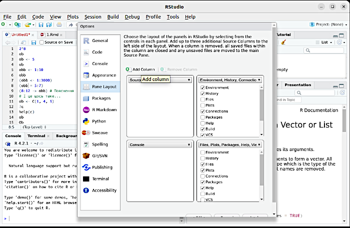

Fig. 2.4.1 Go through the options in the RStudio menu: Tools / Global Options... / Pane Layout / Add Column
In this case, it is convenient to build the code in the second column, in the script editor (Fig. 2.4.2). After the necessary attempts (and in R in general it is quite difficult to get the required text immediately, to open it and to write from scratch; almost always necessary is progression «by feel», through trials and errors) in the script editor, a certain fragment of code can be obtained. After that, this fragment can be transferred to the first column, to the RMarkdown editor, and explained there in any form what, for what purpose, and why exactly this fragment does what it does (without the restrictions imposed on comments in the body of an R-script, where, as you remember, they are created using «hashes» — #).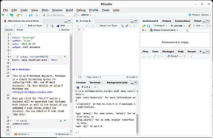

Fig. 2.4.2 This is what the RStudio window looks like in the three-column mode
When RStudio creates an RMarkdown document, it will add the necessary «header» and some explanations. Most of them can be deleted, but it is advisable to leave the first chunk (code fragment). Chunks in RMarkdown are marked with a gray background. The first chunk sets the mode of operation of the following chunks. Let's try to create a new chunk (Fig. 2.4.3).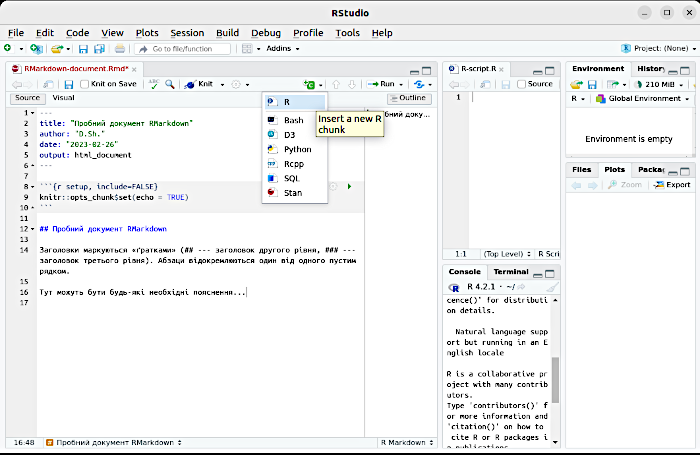

Fig. 2.4.3 To add a chunk, you should «press» the green button with the inscription «+C» and choose its language — in our case R
After the chunk is created, some code fragment can be inserted into it. Fig. 2.4.4 shows how a certain fragment (by the way, as can be seen from the screenshot, written and tested in the script editor) of R-code is inserted into the newly created chunk. This code creates two vectors (ordered sequences), each of 20 elements, and fills these vectors with random sequences of numbers (the first — in the range from 0 to 20, the second — from 0 to 10). After that, R should build a scatter diagram where these random numbers are considered as coordinates of 20 points.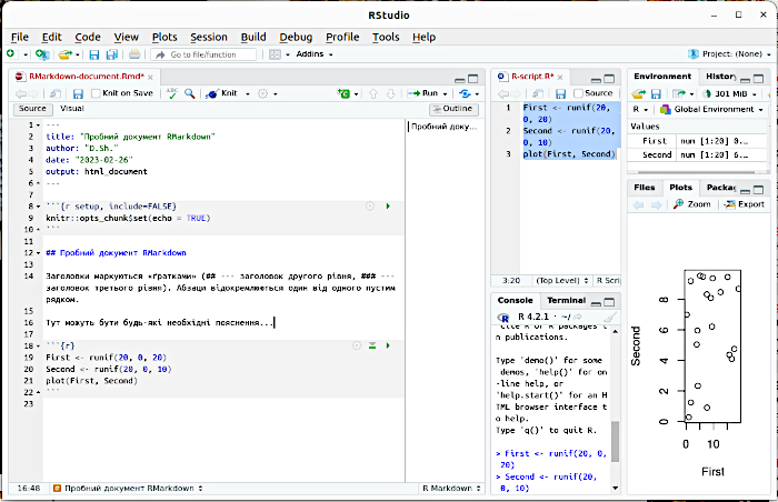

Fig. 2.4.4 The chunk is created. How to execute it?
RMarkdown lines that are not part of chunks create certain marked text. It can be seen if you choose the Visual option in the RMarkdown editor window, instead of the Source option (Fig. 2.4.5).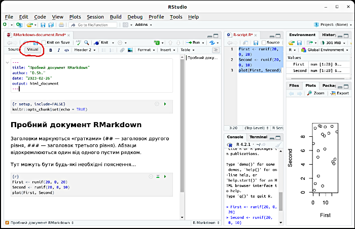

Fig. 2.4.5 Note: the title is shown as a title, the symbols «---» turned into «—». But the appearance of the chunk has not changed significantly
For the R-code in the chunk to be executed, the RMarkdown document should be converted. This is done by the «Knit» button, literally «to bind» (Fig. 2.4.6).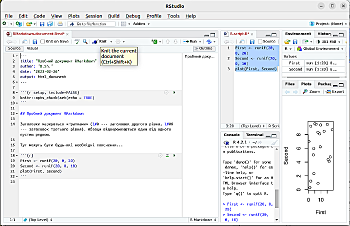

Fig. 2.4.6 The «Knit» button starts converting the RMarkdown document into the specified format
As a result of pressing this button, R will create a new window for the result of converting the text we created. Since in our example the header specifies «output: html_document», a document written in the main language on which internet documents are created, HyperText Markup Language — the hypertext markup language, will be created. A file with the *.html extension will be created automatically. And, as you can see, it will contain both the fragment of R-code that was placed in the chunk, and the result of its execution — the scatter diagram (Fig. 2.4.7).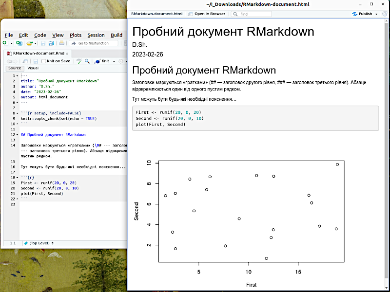

Fig. 2.4.7 The converted *.html document has been created
A «cheat sheet» for RMarkdown can be viewed, for example, here. Some frequently used codes are shown in Fig. 2.4.8. A much more detailed overview is contained, for example, in this book.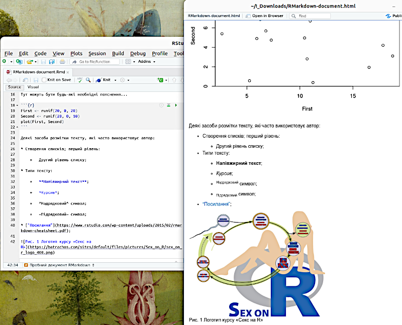

Fig. 2.4.8 Compare the text in the RMarkdown document and in the html document!