

SexOnR–03_ModelTypes. Types of simulation models in the course and their typical structure
Various models that will be created in the course will have much in common. It is necessary to understand how they can be constructed.
Types of simulation models in the course and their typical structure 3.1 Conceptual and implemented simulation models The models we will use in our course will follow several typical patterns. Here we will consider these patterns and build examples of them. This work, which we will do before embarking on the course's planned route, will help us on this route. We will refer to this material throughout all subsequent classes of this course, so do not overlook it! Before creating a simulation model using any software, you should understand what exactly will be modeled and how the sequence of calculations will be built. Simulation modeling is characterized by the use of a certain repeatable set of calculations during each cycle of the model's operation. This cycle can be imagined as obtaining a certain set of calculated values and step-by-step recalculating these values according to defined rules. Thus, when creating a model, you should establish: What exactly should be observed and studied using the model? How should the recalculations of calculated values be structured? What is the input for the model? What set of calculated values does the model work with? According to what rules are recalculations performed during each cycle of the model's operation? How exactly will the model be used? What model operating conditions should be chosen? What are the output data of the model? How will the output data be presented? To answer these questions, you will most likely need to use a certain notation system. This system can be applied when developing and describing the model's calculation algorithm, and then used when describing and presenting research results. An "ideal" conceptual model should be independent of any means of its implementation, for example, R, Python, Excel, or Calc. It could even be independent of computer use. Let's consider a model implemented in a very simple formula – a model in the form of a stack of cards. Imagine a set of cardboard cards on which you can write with a pencil and erase and rewrite these inscriptions in case of recalculation. There are "input" cards; they have input parameters and experimental conditions written on them. To simulate random events, we will use dice rolls. The model's operating algorithm is given by the sequence, conditions, and rules for recalculating cards with calculated values. The model's working cycle is the execution of such a repeatable algorithm and, let's assume, moving cards from one stack to another. Of course, if using a model written in R, this algorithm is defined in the model script; in the case of a "card" model, the algorithm can be defined on a specific group of cards, indicating which card to go to after each step. By the way, is it critically necessary to have a stack of cards, a pencil, and an eraser to implement such a model? No. A sheet of paper and a pencil, or a huge surface of wet clay and a stylus for cuneiform, or a strip of wet sand on the shore are sufficient... Can such models be created? Absolutely. They could have been created several centuries ago. Why weren't they created, say, in the 19th century? They didn't think of it. And such models could help solve quite complex problems. Such models actually have a single (but fatal) drawback – they are extremely inconvenient. Now we can transfer repeatable calculations, which occur according to clearly defined rules, to computers. By the way, the implementation variants of a conceptual model using a set of cards, a clay surface for cuneiform, and a sandy shore have certain peculiarities; different calculation algorithms will likely be optimal for them. Some of the decisions to be made when constructing a conceptual model depend on the specifics of its implementation tool. This also applies to models that will be implemented using software. For example, the R language is vectorized (its basic unit is a sequence of numbers), while Python is not. That is why models optimized for R (and we will consider them further) will have certain peculiarities. 3.2 Typical model structure In general, the various simulation models we will use will consist of a relatively similar set of functional blocks. Here is a possible list for future use; considering models that we will build in this course, if at all, only at the very end. START — BEGINNING : Headline — title ; Explanations — explanations ; Initial script commands — initial script commands (necessary libraries, home directory, reading saved files, initial seed for pseudorandom number generation, clearing the environment, etc.). I. ENTRANCE — INPUT : I.1. Initial state of the system — initial state of the modeled system; I.2. Parameters — parameters by which transformations occur; I.3. Experimental conditions — conditions of the experiment with the model (number of cycles, iterations, etc.); I.4. Changeable parameters combinations — combinations of changeable parameters (in Type III models, where such different combinations are iterated). II. TRANSFORMATIONS SYSTEM CREATION — CREATION OF THE TRANSFORMATION SYSTEM : II.1. Users function setting — creation of user-defined functions, if they are necessary for further calculations; II.2. Parameters combinations mechanism — mechanism for combining changeable parameters (in Type III models); II.3. Objects creation — creation of objects that contain calculated values, accumulate calculation results for further analysis, etc.; if changeable parameters do not affect the created objects, this item can be placed before the previous item; II.4. Calculation rules data — Data with recalculation rules (e.g., tables with crossbreeding results, etc.). III. CALCULATIONS — CALCULATIONS : III.1. Higher level cycles running — running higher-level cycles: iteration cycles, combination of studied parameters, etc.; III.2. Initial composition creation — formation of the initial composition of calculated values depending on input data; III.3. Main work cycle — main work cycle, which in the case of typically complex models is organized as recalculations of certain quantities in stages, denoted by Greek letters: α t N → β t N → γ t N → δ t N → … → ω t N → α t+1 N… ; these recalculations depend on: parameters; experimental conditions; values of other calculated quantities; generated R pseudorandom numbers; III.4. Ending of higher level cycles — ending of higher-level cycles, if necessary – with conditions for early termination of cycles. IV. FINISHING — FINISHING : IV.1. Creating objects for results integration — creation of objects that integrate results (if necessary, for example, for visualization); IV.2. Results saving — saving objects with results ; IV.3. Results viewing — viewing results — main or additional objects or their specific fragments; IV.4. Results visualization — visualization of results ; if necessary – saving visualization results. 3.3 Notation system for work cycle stages and variables adopted in the course In the previous section, when describing the typical structure of models, we noted that in the part of the script we called "III.3. Main work cycle," we will denote stages using Greek letters. Discussing the stages of the cycle and the formulas by which these stages are calculated is a powerful way to describe conceptual and implemented models. Greek letters can be used in R script text, but this leads to a lot of coding confusion. As a result, it is better to insert notations in R scripts where each Greek letter is replaced by two Latin letters. Thus, the first difference between the description of conceptual models and script texts is that in the description, we will use Greek letters, and in scripts – two-letter Latin abbreviations of these letters. The second difference is that in model descriptions, we can use superscript and subscript symbols, while in scripts, this possibility is absent. What we denote as α 1 N when describing the model will look like this in the script: al_1_N . You must start with letters, not numbers, because object names in R cannot start with digits. If the notation for a certain variable quantity needs to indicate which group of individuals it relates to, this group can be indicated in superscripts on the right. For example, if a population consists of individuals a and A, you can use the notation α 1 N a ( al_1_N_a in the script). We have already defined the meaning of superscripts on the left and right, as well as subscripts on the left. One position remains free: subscripts on the right. We will reserve it for denoting the age of individuals; in some population-ecology models, we will have to distinguish between similar groups of individuals that differ in age. In this case, the notation ω 1 N a 2 ( om_1_N_a_2 in the script) should be understood as: the final number of a-individuals of the second age in the first cycle. When describing model algorithms, we will often use a mixed form of recording formulas. In this case, we will insert into R commands not the names of objects that will be used in the script, but the notations that we use to describe this model. For example, when describing the algorithm, we might write: β t N <- α t N + floor( α t N * r + runif(1)) . The formula uses R commands that provide probabilistic rounding (explained in the next section, subsection 3.4.3), combined with the notations for calculated values that we will use when describing models. In the R script text, a similar record would look like this: be_N <- al_N + floor(al_N * r + runif(1)) In some models, we will use more Greek letters than listed in the description of the typical model structure in the previous section. Here is their complete list; in parentheses, we will indicate the two-letter Latin notations that we will use in R scripts: α — alpha (al); β — beta (be); γ — gamma (ga); δ — delta (de); ε — epsilon (ep); ζ — zeta (ze); η — eta (et); θ — theta (th); ι — iota (io); κ — kappa (ka); λ — lambda (la); μ — mu (mu); ν — nu (nu); ξ — xi (xi); ο — omicron (oc); π — pi (pi); ρ — rho (rh); ς — sigma (si); τ — tau (ta); υ — upsilon (up); φ — phi (ph); χ — chi (ch); ψ — psi (ps); ω — omega (om). We will always denote the first stage as α, alpha, and the last, no matter how many individual steps we use in the model, as ω, omega. Why? Because when we engage in simulation modeling, we are actually creating artificial worlds. "I am Alpha and Omega, the First and the Last, the Beginning and the End." Revelation of St. John the Theologian, 22:13. The Bible or Books of the Holy Scripture of the Old and New Testaments. Translation by Ivan Ogienko 3.4 Example of the simplest model: exponential growth 3.4.1 Essence and formulas Among the models describing population processes, the oldest (with a history dating back to the 13th century, from Leonardo Fibonacci) is the exponential growth model; if necessary, you can get additional information about such growth in the textbook "Ecology: Interaction Biology" by D. Shabanov and M. Kravchenko in the section "4.04. Exponential and Logistic Population Growth" . Let's build such a model. The classical growth equation during exponential growth is as follows: dN / dt = r × N , where N is the population size, t is time, and r is the Malthusian parameter, which determines the population's growth capacity. Simulation modeling involves dividing the modeled process into individual steps. The difference equation corresponding to the differential equation for calculating growth is as follows: t+1 N = t N × (1 + r) . We will use this equation. 3.4.2 Implementation in R We will use far from all the elements of the model structure compared to those listed in section 3.2. It is clear that this is a consequence of the relative simplicity of the discussed model.
# ЕКСПОНЕНЦІЙНЕ ЗРОСТАННЯ
# «Мінімальна» модель, що зроблена для демонстрації принципу роботи імітаційних моделей та робочого циклу
# I. ENTRANCE — ВХІД:
# Initial state of the system — початковий стан модельованої системи
al_0_N  <- 10 # Початкова чисельність модельної популяції
# Parameters — параметри
r <- 0.05 # Параметр Мальтуса, приріст чисельності на кожному кроці
# Experimental conditions — умови експерименту з моделлю
cycles <- 50 # I.3 Кількість циклів
# II TRANSFORMATIONS SYSTEM CREATION — СТВОРЕННЯ СИСТЕМИ ПЕРЕТВОРЕНЬ:
# Objects creation — створення об’єктів
N <- rep(NA, cycles+1) # Створення вектору для розрахунків та збору результатів (у цьому випадку ці дві задачі вирішує тій самий вектор)
names(N) <- 0:cycles # Кожне значення у векторі N отримає своє ім'я; перше по рахунку буде позначено як 0: початкове значення N
# III. CALCULATIONS — РОЗРАХУНКИ:
# Initial composition creation — утворення початкового складу
N[1] <- al_0_N # Перше значення (з ім'ям 0) визначається відповідно до початкового стану
# Main work cycle — основний робочий цикл
for (t in 1:cycles) { N[t+1] <- floor(N[t] * (1 + r) + runif(1)) } # Робочий цикл моделі повторює робочу формулу таку кількість разів, яка визначена умовами експерименту. Результат перерахунку залежить від значення розрахункової величини (попереднього значення в векторі), параметру (що визначає швидкість зростання популяції), умов експерименту (кількості кроків, яку відраховує лічильник у циклі) та випадкової величини(визначає ймовірнісне скорочення отриманої величини до цілих значень)
# IV. FINISHING — ЗАВЕРШЕННЯ:
# Results viewing — перегляд підсумків
N # Результати збережені в векторі N; на них можна просто подивитися
##   0   1   2   3   4   5   6   7   8   9  10  11  12  13  14  15  16  17  18  19
##  10  10  11  11  11  11  12  13  14  15  16  17  18  19  20  21  22  24  25  26
##  20  21  22  23  24  25  26  27  28  29  30  31  32  33  34  35  36  37  38  39
##  27  28  29  30  32  33  35  36  38  39  41  43  46  49  52  55  58  61  64  67
##  40  41  42  43  44  45  46  47  48  49  50
##  70  73  76  80  84  88  92  96 101 106 111
# Results visualization — візуалізація підсумків
plot(N) # Ця команда виводить результати на найпростіший графік
Fig. 3.4.2.1 Visualization of the exponential growth model 3.4.3 Probabilistic rounding Let's provide some comments on the constructed model. Let's consider that the applied equation can give non-integer values. When it comes to population size, this does not have a clear biological meaning. Rounding should be used. Which one? The standard rounding method is not always suitable.
round(3.3)
## [1] 3
round(3.4999)
## [1] 3
round(3.5)
## [1] 4You see that there is a certain threshold that clearly separates the rounded values. Does this make biological sense? Try running the model above with the following snippet:
# Main work cycle — основний робочий цикл
for (t in 1:cycles) { N[t+1] <- round(N[t] * (1 + r)) }
What is the output? A constant population size. But that shouldn't be the case, should it? Probabilistic rounding makes more biological sense. A random variable uniformly distributed between 0 and 1 is added to the rounded value. Then the fractional part is rounded down (the nearest integer value is taken).
ProbabRound <- rep(NA, 1000)
for (i in 1:1000) {ProbabRound[i] <- floor(3.3 + runif(1))}
mean(ProbabRound)
## [1] 3.316With probabilistic rounding, 3.3 will be rounded up to 4 in three out of ten cases and down to 3 in seven out of ten. In the example above we computed the mean of 1000 such trials. It varies from run to run but is usually close to 3.3.
In our view, probabilistic rounding has the greatest biological sense.
al_0_N  <- 10
r <- 0.05
cycles <- 50
N <- rep(NA, cycles+1)
names(N) <- 0:cycles
N[1] <- al_0_N
for (t in 1:cycles) { N[t+1] <- floor(N[t] * (1 + r) + runif(1)) }
plot(N, main = "Exponential growth", xlab = "Generations", ylab = "Population size")
Fig. 3.4.4.1 Captions were added to the visualization. When it comes to such simple models, they (with some experience) are not difficult to understand without comments in the script. However, even in this course, we will have to deal with much more complex models, which are extremely difficult for even their author to understand without explanations in the script itself. To better understand the logic of the described model, it can be represented as a diagram. Fig. 3.3.4.1 The structure of the described simplest model can be represented graphically as follows. Try to match the textual description of the typical model structure (section 3.2), the example of the simplest model in R (section 3.4.2), and the graphical diagram! We will not classify the model described in section 4.4 into any type. The fact is that for the purposes of our course, such models are not useful. We built this model as a simulation model and used difference equations for this. However, usually such problems are solved differently: analytical models are built on differential equations. This model was built solely to show the structural parts of a simulation model with the simplest possible example. 3.5 Type I Model: Determining Process Dynamics from a Certain Number of Cycles Consisting of Stages 3.5.1 Building a Conceptual Model and a System of Stage Notation in a Cycle Now let's move on to a model that better suits the goals of our course. Let's denote it as Type I model (there will be Type II models consisting of many Type I models, and Type III models consisting of many Type II models ahead!). In the exponential growth model, the cycle consisted of a single action. This is an atypical case for simulation modeling. Now we will build a cycle consisting of several actions. To not deviate from the canon, after the exponential model, we will build a logistic one. The logistic equation in difference form looks like this: t+1 N = t N × (1 + r) × ( K– t N / K ) , where N is the population size, t is time, r is the Malthus parameter determining the population's growth capacity, and K is the Verhulst parameter setting the population size limit. This equation could have been reflected in the model we built in section 3.4; it would have been enough to add K to the parameters and slightly complicate the formula of the working cycle. But we will build a more complex model. Let's consider the lifespan of individuals in it (denote it max a , or max_a in the R-model text). How to simulate lifespan limitation? At each step of the model, subtract from the population size the number of individuals that were added to it max a steps ago. Now, in the working cycle, we have to simulate two processes: the death of old individuals and the reproduction of existing ones. Is it worth combining these two processes in one formula? No. It is inconvenient and not clear. It will be good if we build a model that is easy to understand, for which step-by-step verification is possible, and which is easier to complicate by adding new elements to it. We will need a system of notation. We will denote the stages in the cycle using Greek letters, and the cycles themselves with numbers. Let's make a slight change in notation compared to the exponential growth model. In that model, we characterized the model population in cycle t as t N (meaning N - number). If the model population consists of individuals identical (from the modeling point of view), it can be characterized simply by its size. If we consider the age of individuals, the model population becomes heterogeneous for us; we will denote it t P (P - population). Let's distinguish four stages in the cycle: Alpha population, α P , the set of individuals at the beginning of the cycle; in the first cycle, it depends on the initial composition specified in the input parameters: α 1 P = al_1_N , and subsequently it is determined by the omega population of the previous cycle: α t+1 P = ω t P ; Beta population, β P , the set of individuals after the death of individuals of maximum age, β t+max_a P = α t+max_a P – γ t P ; Gamma (sub)population, γ P , offspring: γ t P = β t P × (1 + r) × (K – β t P) / K ; Omega population, ω P , the final size in the cycle: ω t P = β t P + γ t P . 3.5.2 R-model of logistic growth considering mortality at a certain age
# ЛОГІСТИЧНЕ ЗРОСТАННЯ З ВРАХУВАННЯМ СМЕРТНОСТІ У ПЕВНОМУ ВІЦІ (Модель І типу)
# Робочий цикл: альфа-популяція → загибель старших за max_a особин →
# → бета-популяція → логістичне розмноження → гама (приплід) → омега → альфа
# I. ENTRANCE — ВХІД:
# Initial state of the system — початковий стан модельованої системи
al_1_N  <-  10 # Початкова чисельність модельної популяції
# Parameters — параметри
r <- 0.3 # Параметр Мальтуса, приріст чисельності на кожному кроці
K <- 500 # Параметр Ферхюльста, що задає обмеження чисельності популяції
max_a <- 5 # Тривалість життя особини (у циклах)
# Experimental conditions — умови експерименту з моделлю
cycles <- 100 # Кількість циклів
# TRANSFORMATIONS SYSTEM CREATION — СТВОРЕННЯ СИСТЕМИ ПЕРЕТВОРЕНЬ:
# Objects creation — створення об’єктів
al_P <- rep(NA, cycles+1) # Вектор для початкової (на кожному циклі) чисельності
ga_P <- rep(NA, cycles) # Вектор для потомства
# III. CALCULATIONS — РОЗРАХУНКИ:
# Initial composition creation — утворення початкового складу
al_P[1] <- al_1_N # Перше значення визначається відповідно до початкового стану
# Main work cycle — основний робочий цикл
for (t in 1:cycles) { # Початок робочого циклу
  if(t < max_a) be_P <- al_P[t] # Усі особини ще «молоді», усі лишаються живі
  if(t == max_a) be_P <- al_P[t] - al_P[1] # Гине початковий склад популяції
  if(t > max_a) be_P <- al_P[t] - ga_P[t-max_a] # Гине приплід, утворений max_a циклів тому
  ga_P[t] <- floor(be_P * r * (K - be_P) / K + runif(1)) # Приплід
  om_P <- be_P + ga_P[t] # Прикінцевий склад
  al_P[t+1] <- om_P # Перехід на наступний цикл роботи моделі
} # Кінець робочого циклу
# IV. FINISHING — ЗАВЕРШЕННЯ:
# Results viewing — перегляд підсумків
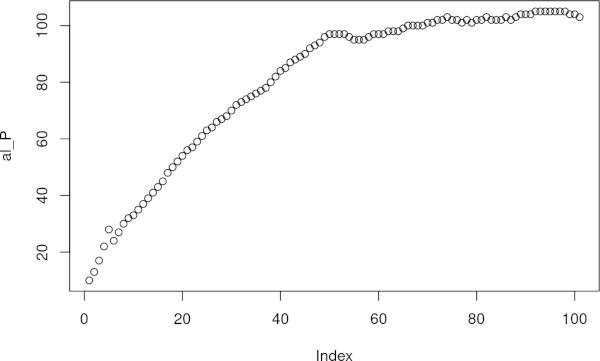
al_P # Результати збережені в векторі al_P; на них можна просто подивитися
##   [1]  10  13  16  20  26  20  21  23  24  23  24  26  27  29  31  33  34  36
##  [19]  37  39  41  43  44  46  48  50  52  55  57  58  60  62  64  66  68  70
##  [37]  72  74  76  78  80  81  82  83  84  84  86  87  89  90  91  92  93  93
##  [55]  94  95  95  95  96  97  98  99 101 102 103 103 103 103 102 102 103 104
##  [73] 103 104 103 102 102 102 101 101 102 101 102 103 104 104 105 105 104 103
##  [91] 103 103 102 102 103 102 102 102 102 101 101
# Results visualization — візуалізація підсумків
plot(al_P, main = "Logistic growth", xlab = "Generations", ylab = "Population size") # Графік
Alpha‑population, αP, the set of individuals at the beginning of the cycle; in the first cycle it depends on the initial composition given in the input parameters: α1P = al_1_N, and thereafter is defined by the omega‑population of the previous cycle: αt+1P = ωtP;
Omega‑population, ωP, the final size in the cycle: ωtP = βtP + γtP.
3.5.3 Scheme of the organization of the considered Type I model (logistic growth)
As before, we will use a scheme to show how our model is organized.
The main novelty of this scheme, compared with the previous one, is that it shows the organization of recalculations as repetitions of certain cycles composed of stages.
3.6 Model Type II: establishing the probability distribution of results for a group of iterations with identical parameters
3.6.1 Purpose of the Type II model
As you know, models can be deterministic and nondeterministic (including stochastic, random elements). When we can clearly and confidently specify all factors influencing the expected outcome, deterministic models can be used. More often, however, the full set of factors is unknown and it is impossible to precisely determine their strengths…
In fact, even the example of analytical modelling shown on the slide is characterized by a number of unknown factors. It is impossible to mathematically determine the exact point where an artillery shell will land. Nevertheless, for practical purposes this is unnecessary; it is enough that the weapon hits the target, and this can be achieved even if it lands a short distance from the target. It is important to remember that any model contains a certain degree of uncertainty (and sometimes it is akin to coffee‑ground divination).
Suppose, using the Type I model we established some dynamics of the studied system. So what? How much can we trust the result? Is it a regular consequence of the factors we considered, or does it reflect a low‑probability event? To determine this, modelling should be repeated, not just once. Repetitions with the same parameters are characteristic of Type II models, and with varying parameters—for Type III models.
Of course, to find out whether we always obtain the same result, a single Type I model would suffice. We could simply run it repeatedly and record the outcomes. But why do this “manually” when it can be done by a slight restructuring of the model itself?
By moving from a Type I to a Type II model we shift from a single observation of a model experiment result to the ability to analyse the probability distribution of results.
# ЛОГІСТИЧНЕ ЗРОСТАННЯ З ВРАХУВАННЯМ СМЕРТНОСТІ У ПЕВНОМУ ВІЦІ (Модель ІІ типу)
# Група ітерацій. Робочий цикл: альфа-популяція → загибель старших за max_a особин →
# → бета-популяція → логістичне розмноження → гама (приплід) → омега → альфа
# I. ENTRANCE — ВХІД:
# Initial state of the system — початковий стан модельованої системи
al_1_N  <-  5 # Початкова чисельність модельної популяції
# Parameters — параметри
r <- 0.3 # Параметр Мальтуса, приріст чисельності на кожному кроці
K <- 500 # Параметр Ферхюльста, що задає обмеження чисельності популяції
max_a <- 5 # Тривалість життя особини (у циклах)
# Experimental conditions — умови експерименту з моделлю
cycles <- 100 # Кількість циклів
iterat <- 10 # Кількість ітерацій
# II. TRANSFORMATIONS SYSTEM CREATION — СТВОРЕННЯ СИСТЕМИ ПЕРЕТВОРЕНЬ:
# Objects creation — створення об’єктів
al_P <- rep(NA, cycles+1) # Вектор для початкової (на кожному циклі) чисельності
ga_P <- rep(NA, cycles) # Вектор для потомства
Rezult <- matrix(NA, nrow = cycles+1, ncol = iterat) # У разі використання ітерацій, потрібна матриця, а не вектор, як у моделі І типу
# III. CALCULATIONS — РОЗРАХУНКИ:
# Higher level cycles running — запуск циклів вищого рівня
for (i in 1:iterat) { # Початок ітерації
# Initial composition creation — утворення початкового складу
  al_P[1] <- al_1_N # Перше значення визначається відповідно до початкового стану...
  Rezult[1, i] <- al_1_N # ...і зберігається в матриці для результатів
# Main work cycle — основний робочий цикл
  for (t in 1:cycles) { # Початок робочого циклу
  if(t < max_a) be_P <- al_P[t] # Усі особини ще «молоді», усі лишаються живі
  if(t == max_a) be_P <- al_P[t] - al_P[1] # Гине початковий склад популяції
  if(t > max_a) be_P <- al_P[t] - ga_P[t-max_a] # Гине приплід, утворений max_a циклів тому
    ga_P[t] <- floor(be_P * r * (K - be_P) / K + runif(1)) # Приплід
    om_P <- be_P + ga_P[t] # Прикінцевий склад
    al_P[t+1] <- om_P # Перехід на наступний цикл роботи моделі
    Rezult[t+1, i] <- al_P[t+1]
                       } # Кінець робочого циклу
  # Ending of higher level cycles — завершення циклів вищого рівня
                     } # Кінець циклу ітерацій
# IV. FINISHING — ЗАВЕРШЕННЯ:
# Results viewing — перегляд підсумків
head(Rezult) # Підсумки збережені в цій матриці; можна подивитися на її «голову» (початок)...
##      [,1] [,2] [,3] [,4] [,5] [,6] [,7] [,8] [,9] [,10]
## [1,]    5    5    5    5    5    5    5    5    5     5
## [2,]    7    6    7    6    6    7    7    6    6     6
## [3,]    9    8    9    8    8    9    9    8    8     8
## [4,]   12   10   12   10   10   12   12   11   11    11
## [5,]   15   12   15   12   13   16   16   14   14    14
## [6,]   13    9   13    9   10   14   14   12   11    12
tail(Rezult) # ...та «хвіст» (кінець)
##        [,1] [,2] [,3] [,4] [,5] [,6] [,7] [,8] [,9] [,10]
##  [96,]  101  104  105  105  104  103  105  101  102   103
##  [97,]  100  105  105  105  104  103  105  101  102   103
##  [98,]  100  105  104  105  104  103  105  102  102   102
##  [99,]  100  105  104  105  104  102  105  102  103   101
## [100,]  100  105  103  105  104  103  105  101  102   100
## [101,]  100  105  103  105  105  103  105  101  103   101
# Results visualization — візуалізація підсумків
plot(Rezult[, 1], type="l", lty=1, col="red", ylim=c(0, 110),
     main = "Dynamics of the model population\nin 10 different iterations",
     xlab="Simulation cycles", ylab="Amount of the model population")
lines(Rezult[, 2], type="l", lty=1, col="blue")
lines(Rezult[, 3], type="l", lty=1, col="brown")
lines(Rezult[, 4], type="l", lty=1, col="chartreuse")
lines(Rezult[, 5], type="l", lty=1, col="coral")
lines(Rezult[, 6], type="l", lty=1, col="darkviolet")
lines(Rezult[, 7], type="l", lty=1, col="gold")
lines(Rezult[, 8], type="l", lty=1, col="deepskyblue")
lines(Rezult[, 9], type="l", lty=1, col="hotpink")
lines(Rezult[, 10], type="l", lty=1, col="lightsalmon")
Fig. 3.6.2.1 Result of Type II model operation. We see 10 separate simulations We won't look for complex visualization methods now and will limit ourselves to plotting 10 separate growth curves of the model population. Now we see that the dynamics of the model population, despite the influence of randomness, are quite regular. However, this is not always the case; we will still see models where different iterations with the same initial conditions lead the model population to fundamentally different states. 3.6.3 Organizational Scheme of the Discussed Type II Model As in the previous cases, we will provide a diagram showing how the discussed model works. We see a "stack" of iterations, each corresponding to a Type I model. Each of them is influenced by a set of input values, parameters, and conditions. Based on the comparison of outputs from each iteration, an analysis of the probability distribution of modeling results for the given parameters is performed. Fig. 3.6.3.1 Diagram showing the structure of the described Type II model We used the simplest method of analyzing probability distributions: comparing a group of curves. Of course, there are more complex and sophisticated ways to solve this problem. 3.7 Type III Model: Establishing the Influence of Parameters on the Modeling Result 3.7.1 Purpose of Type III Model The use of simulation models can be justified in various ways. However, for the author of this course, the sense related to finding answers to a series of closely related questions is more important: can the observed behavior (dynamics, traits) of natural systems be a consequence of a certain mechanism? Is the interaction between a set of factors assumed by a certain hypothesis sufficient to explain the observed properties of natural systems? Under what conditions can a certain set of factors cause the phenomena we observe? How does a change in a specific factor affect the behavior of the studied system, assuming our hypotheses about its functioning mechanisms are correct? To answer these questions, using a Type II model is insufficient. Suppose we have determined the probability distribution of the output states of the model system for a given set of input parameters. But can we be sure, without verification, that the system will behave similarly under different conditions? Consider that we use models precisely in cases where the behavior of the studied system is non-trivial, when its study requires considering the interaction between a specific set of factors. What to do? Perhaps we haven't found answers to our questions simply because we chose unfavorable input parameters for our Type II model? We should check the behavior of the model system under different input parameter values. How to do this – manually? It's possible manually, but since we are dealing with a computer model, it is rational to entrust it with the methodical verification of all necessary combinations of studied parameters and processing the obtained results. When dealing with changes in two independent parameters (and this is the case we will consider), the results of combining combinations can be visualized. If more parameters need to be changed, determining the research outcome may involve establishing at which input parameter values a certain function reaches its maximum or minimum. It should be considered that iterating through too many input parameters can lead to a catastrophic increase in computation time. Sometimes it makes sense to conduct "reconnaissance" with a small number of iterations for each combination of input parameters, and only after identifying areas of interest in the combination space, study them in more detail and with higher quality. 3.7.2 Modifying Type II Model into Type III Model In the Type III model, we will have to "stretch" two more cycles over the two existing cycles in the Type II model: for each of the varying parameters. Overall, compared to the Type II model, the following changes are necessary (we will vary the Malthus parameter and the maximum age of individuals): an additional library for 3D graphics, plot3D, will be used for visualizing results; in this case, this library should be activated at the beginning of the model's operation, and if it is not installed on the system, it should be installed beforehand (in the given example, the installation command is commented out with a '#'); commands that set constant values for parameters that will be changed should be removed or commented out; vectors (vector_r and vector_max_a) should be defined, containing the values of the varying parameters that will be combined; since the Result matrix, which collected the iteration results, works only with a specific combination of varying parameters, an object should be created to collect an integrating quantity (i.e., a quantity that reflects changes important to the experimenter in the studied system), which will characterize the result of each group of iterations; let's call such a matrix Outcome; the average population size at the end of each iteration, when its size reaches equilibrium and its fluctuations become random, can be used as the integrating quantity; the command Outcome[a, b] <- mean(Rezult[(cycles-20):(cycles+1), ]) will ensure the recording of the average value from 21 consecutive final population size states in each iteration; visualization of results using the persp3D function will allow viewing the overall result.
# ЛОГІСТИЧНЕ ЗРОСТАННЯ З ВРАХУВАННЯМ СМЕРТНОСТІ У ПЕВНОМУ ВІЦІ (Модель ІІІ типу)
# Визначення рівноважної чисельності популяцій в групах ітерацій за різної тривалості життя
# та швидкості розмноження. Робочий цикл: альфа-популяція → загибель старших за max_a особин →
# → бета-популяція → логістичне розмноження → гама (приплід) → омега → альфа
# Initial script commands — початкові команди скрипту
# install.packages("plot3D") # Інсталяція пакету 3D-візуалізації (достатньо виконати 1 раз)
library(plot3D) # Активація пакету (необхідно виконувати кожного разу)
# setwd("~/data/SexOnR") # Робоча директорія (лише для Д.Ш.!!!)
rm(list = ls()) # Очищення раніше збережених об'єктів в Environment
# set.seed(123456) # Забезпечення повторюваності у виборі псевдовипадкових чисел
# I. ENTRANCE — ВХІД:
# Initial state of the system — початковий стан модельованої системи
al_1_N  <-  5 # Початкова чисельність модельної популяції
# Parameters — параметри
# r <- 0.3 # Параметр Мальтуса, приріст чисельності на кожному кроці; ЗМІНЮВАНИЙ ПАРАМЕТР!
K <- 500 # Параметр Ферхюльста, що задає обмеження чисельності популяції
# max_a <- 5 # Тривалість життя особини (у циклах); ЗМІНЮВАНИЙ ПАРАМЕТР!
# Experimental conditions — умови експерименту з моделлю
cycles <- 150 # Кількість циклів
iterat <- 20 # Кількість ітерацій
# Changeable parameters combinations — комбінації змінюваних параметрів
# Створення векторів зі значеннями змінних параметрів, які будуть перебиратися у ході роботи:
vector_r <- c(0.1, 0.2, 0.3, 0.4, 0.5, 0.6) # Варіанти значень параметру Мальтуса
vector_max_a <- c(2, 3, 4, 5, 6, 7) # Варіанти максимальної тривалості життя
# II TRANSFORMATIONS SYSTEM CREATION — СТВОРЕННЯ СИСТЕМИ ПЕРЕТВОРЕНЬ:
# Parameters combinations mechanism — механізм комбінації змінюваних параметрів
Outcome <- matrix(NA, nrow = length(vector_r), ncol = length(vector_max_a), dimnames = list(vector_r, vector_max_a)) # Кожна комірка цієї матриці відповідає певній комбинації змінюваних параметрів
# Цикли, що перебирають досліджувані сполучення параметрів:
for (a in 1:length(vector_r)){ # Цикл, що змінює значення параметру Мальтуса
  r <- vector_r[a] # Змінюване значення чисельності популяції
  for (b in 1:length(vector_max_a)){ # Цикл, що змінює максимальну тривалість життя
    max_a <- vector_max_a[b] # Змінюване значення сили добору
    # Objects creation — створення об’єктів
    al_P <- rep(NA, cycles+1) # Вектор для початкової (на кожному циклі) чисельності
    ga_P <- rep(NA, cycles) # Вектор для потомства
    Rezult <- matrix(NA, nrow = cycles+1, ncol = iterat) # Матриця для збору результатів ітерацій з певною комбінацією параметрів
    # III. CALCULATIONS — РОЗРАХУНКИ:
    # Higher level cycles running — запуск циклів вищого рівня
    for (i in 1:iterat) { # Початок ітерації
      # Initial composition creation — утворення початкового складу
      al_P[1] <- al_1_N # Перше значення визначається відповідно до початкового стану
      Rezult[1, i] <- al_1_N
      # Main work cycle — основний робочий цикл
      for (t in 1:cycles) { # Початок робочого циклу
    if(t < max_a) be_P <- al_P[t] # Усі особини ще «молоді», усі лишаються живі
    if(t == max_a) be_P <- al_P[t] - al_P[1] # Гине початковий склад популяції
    if(t > max_a) be_P <- al_P[t] - ga_P[t-max_a] # Гине приплід, утворений max_a циклів тому
        ga_P[t] <- floor(be_P * r * (K - be_P) / K + runif(1)) # Приплід
        om_P <- be_P + ga_P[t] # Прикінцевий склад
        al_P[t+1] <- om_P # Перехід на наступний цикл роботи моделі
        Rezult[t+1, i] <- al_P[t+1]
                           } # Кінець робочого циклу
      # Ending of higher level cycles — завершення циклів вищого рівня
                         } # Кінець циклу ітерацій
    Outcome[a, b] <- mean(Rezult[(cycles-20):(cycles+1), ]) # Запис певного значення у матрицю зі сполученнями параметрів
                                    } # Кінець циклу, що змінює максимальну тривалість життя
                              } # Кінець циклу, що змінює значення параметру Мальтуса
# IV. FINISHING — ЗАВЕРШЕННЯ:
# Results saving — збереження об’єктів з результатами
# save(Outcome, file = "Outcome.RData")
# Results visualization — візуалізація підсумків
persp3D(z = Outcome, x = vector_r, y = vector_max_a, theta = 330, phi = 30, # Побудова графіку
        xlab = "r", ylab = "max_a",
        expand = 0.8, facets = FALSE, scale = TRUE,  ticktype = "detailed",nticks = 6, cex.axis=0.9,
        clab = "mean N", colkey = list(side = 2, length = 0.5))
Fig. 3.7.2.1 Result of Type III model operation. We see how the model population size (mean N) depends on the lifespan of individuals (max_a) and their reproductive potential, i.e., the number of offspring (r) The three-dimensional visualization we are creating has drawbacks regarding label placement, but it reflects an important result: both reproductive potential and lifespan significantly influence the level at which the model population size stabilizes. Pay attention to the placement of curly braces in the provided script. The course author prefers when the closing brace of a cycle or another group of commands is located below the opening brace of that cycle or group. 3.7.3 Organizational Scheme of the Discussed Type III Model As in the previous sections of this chapter, we will conclude the discussion of the model with a diagram. It shows only the main elements of the model; if this diagram were sufficiently detailed, it would become cumbersome and difficult to perceive. The diagram shows a table, the cells of which correspond to different combinations of the studied parameters. Within each such cell is effectively a Type II model. The output of each such model is no longer a probability distribution, but a single value. The values of such a quantity can become, for example, individual areas that form a three-dimensional surface. This surface will reflect the dependence of the modeling result on the parameter values. Of course, the informativeness and usefulness for understanding processes of such a model are much higher than those of the previous ones. Fig. 3.7.3.1 Diagram showing the structure of the described Type III model Of course, it is not mandatory that Type III models study changes in exactly two parameters. Three parameters are too many; it is unclear how to visualize the result. One parameter is entirely possible, and a standard graph (with the studied parameter's value on the x-axis and the integrating quantity characterizing the modeling result on the y-axis) is a perfectly acceptable way to present the results of such a study. 3.8 Some Features of R Models 3.8.1 Appearance of an R Script The author of this text must admit to having a very poor memory for specific details related to models and R scripts in general. When writing them, even the simplest R commands have to be looked up in various cheat sheets. The memory for specific ways to solve one problem or another is lost very quickly. When, after a month or two, one has to look at their own R script, it appears unfamiliar... When writing a script, one has to try different sequences of commands. The author usually leaves them after the main text of the script. When exploring possibilities, one writes as quickly as possible without any explanations, using single-letter object names. Whether a solution was found or not – after a while, looking at these attempts, it becomes impossible to understand anything. What was saved "for the future" without explanation turns out to be useless. How to reduce the destructive effect of such rapid forgetting? Pay significant attention to the appearance of the script. An example of how the author does this (when he has time to be meticulous about the results of his own work) is the previous R code fragment. What features are worth noting? The script contains many comments. Some comments are placed after R commands on the same line, some are before the working line (if they explain what is happening in the next line, they end with a colon). The script has a header. Objects have meaningful names (Result, Outcome, etc.) or are formed according to clear rules (Al_Pop, Be_Pop, Ga_Pop, Om_Pop, al_1_N_a, al_1_N_A), which correspond to the notations in the model description (α P, β P, γ P, ω P, α 0 P a, α 0 P A respectively). Lines belonging to a specific cycle or condition are indented, showing their dependency on the lines where these functions (for, if, etc.) begin. The closing curly brace of a cycle is located exactly or approximately at the level of the opening curly brace of that cycle. Spaces are intentionally placed in the script text to facilitate its readability. Spaces are placed before and after assignment symbols <-, equals signs =, and hash symbols #, after commas and semicolons. Symbols + , - etc. are placed between spaces if they combine relatively complex names (e.g., (length(which(Al_Pop==1)) + length(which(Al_Pop==0)) )), and without spaces in case of short names ( Rezult[cycles+1, i] ). The author is not a neat person in everyday life. At home, he has to listen to his wife's remarks, and at work – from graduate students and management for not putting things in their places. However, experience with data files in statistics, with simulation models in spreadsheets and in R has taught him neatness and attention to detail in these matters. The effort you put into making your scripts clearer will pay off handsomely by saving your own time when you return to your models, and will offer a faint hope that others will understand you better. 3.8.2 Beginning of an R Document The beginning of an R document may not contain any additional elements (the previously provided R code fragment is fully functional!), or it may start with a few useful commands. In many cases, R models use the capabilities of additional packages. These packages should be installed once on the computer where R is running, and activated each time the model is launched. The following commands are used for this purpose.
# install.packages("plot3D") # Інсталяція пакету 3D-візуалізації (достатньо виконати 1 раз)
library(plot3D) # Активація пакету (необхідно виконувати кожного разу)
The package installed by the first command and activated by the second will be needed for visualizing the results of the model we created. After this package is installed, the first command can be commented out with a '#'. When R is used to solve several different tasks on a user's computer, the results of the work can become mixed up. It is often convenient to divide them into separate folders (directories). Naturally, the path to the working directory is specific to each user.
setwd("~/data/SexOnR") # Робоча директорія (лише для Д.Ш.!!!)The method of writing the path to the working directory differs across operating systems (the previous example shows a variant typical for Linux; in Windows, the address looks different). To determine how to write the working directory address, you can set it "manually" (go to the Files menu, select the desired folder, and execute the command More / Set As Working Directory). In the RStudio console, as shown in the figure, the corresponding command will appear (RStudio will "translate" the selection made with the cursor into R command language in the correct format). Fig. 3.8.2.1 After selecting the Set As Working Directory option, the corresponding command appeared in the RStudio console. When running the same script or similar scripts repeatedly, there is a certain danger. In the program's workspace, in the Environment, certain objects are created. In a subsequent run of the script or its fragment, one might not notice that a previously created object is being used in the calculations. This is one of the possible sources of errors. To prevent this from happening, a command can be inserted at the beginning of the script to clear the Environment – the "space" where commands are executed. Of course, one can choose not to use the provided command and clear the Environment "manually".
rm(list = ls()) # Очищення раніше збережених об'єктів в EnvironmentThis lecture is written in R Markdown. If you are working with a Markdown document (it has a *.Rmd extension), all R calculations will be redone when you run it. If the model is non-deterministic, i.e., uses random numbers, you will see different results than the author sees. There are also more important cases where it is desirable to make the results of R work predictable. Suppose you have created a model. When running it, it sometimes produces errors – and sometimes it doesn't. Errors are related to a specific combination of calculated values in the model... To investigate this situation step by step, you need to review the intermediate calculation results to understand where something went wrong. But with each run, R will select different pseudo-random numbers for calculations. What to do? "Freeze" the starting point of pseudo-random number calculations. This can be done using the set.seed() command; enter any number in the parentheses.
# set.seed(123456) # Забезпечення повторюваності у виборі псевдовипадкових чиселNow, calculations with random numbers will lead to the same result every time. Another important addition to the main "body" of the program can be commands for saving and reading the results of long calculations. Suppose our calculations involved calculating the Outcome matrix for a long time. To use it later, it is rational to save it as a separate file. If the path to a specific directory is not specified, this file will be saved in the working directory that the script is operating with. After creating the Outcome matrix, we could save it.
# save(Outcome, file = "Outcome.RData")The saved file containing the Outcome matrix can be read using the command load("Outcome.RData"). // add bootstrap table styles to pandoc tables function bootstrapStylePandocTables() { $('tr.odd').parent('tbody').parent('table').addClass('table table-condensed'); } $(document).ready(function () { bootstrapStylePandocTables(); }); $(document).ready(function () { window.buildTabsets("TOC"); }); $(document).ready(function () { $('.tabset-dropdown > .nav-tabs > li').click(function () { $(this).parent().toggleClass('nav-tabs-open'); }); }); (function () { var script = document.createElement("script"); script.type = "text/javascript"; script.src = "https://mathjax.rstudio.com/latest/MathJax.js?config=TeX-AMS-MML_HTMLorMML"; document.getElementsByTagName("head")[0].appendChild(script); })();