SexOnR–10_Sturtevant. Modelling Cyclically Varying Selection according to Sturtevant and Others (Assignment II)
One of the ideas put forward to explain the Maynard Smith paradox simply calls out to be investigated using simulation modelling. This idea belongs to Alfred Sturtevant and was developed (simplified) by William Hamilton and Alexei Kondrashov
One of the possible mechanisms that could ensure the maintenance of sexual reproduction in populations was proposed by Alfred Sturtevant. Sturtevant's model concerned epistatic selection that initially favoured certain gene combinations, then others. The name of epistatic selection according to Sturtevant is connected with the phenomenon of epistasis — gene interaction. William Hamilton and Alexei Kondrashov realized that this mechanism should also operate in the case of changes in the nature of selection in favour of different allele combinations at the same gene. The nature of selection considered by Hamilton and Kondrashov can be called cyclically varying.
The logic of this process is shown in the table.
Table 8.1.1 Cyclically varying selection that alternately favours heterozygotes and homozygotes
|
Generation |
Nature of selection |
AA |
Aa |
aa |
|
Genotypes |
||||
|
1 |
odd: homozygotes are eliminated |
|
Aa |
|
|
2 |
even: heterozygotes are eliminated |
AA |
|
aa |
|
3 |
odd: homozygotes are eliminated |
|
Aa |
|
|
4 |
even: heterozygotes are eliminated |
AA |
|
aa |
|
… |
… |
|||
This idea is worth testing using a simulation model. At the beginning of such a study, one can verify that the described mechanism will indeed promote sexual reproduction in sexually reproducing organisms and hinder parthenogens. It is interesting to determine what selection compensates for the «twofold cost of sex». In addition, it is interesting to verify whether the assumption is correct that cross-fertilizing hermaphrodites will be the most successful under such conditions.
|
Coding of genotypes and modes of reproduction of individuals in the model |
Genotypes |
|||||
|
Homozygote for the dominant allele |
Heterozygote |
Homozygote for the recessive allele |
||||
|
AA |
Aa |
aa |
||||
|
+0.11 |
+0.12 |
+0.22 |
||||
|
Mode of reproduction |
Females |
Fe |
1+ |
1.11 |
1.12 |
1.22 |
|
Thus, the obtained results reflect the trend of the HPS returning to the state recorded by G.A. Lada in 1995 [3;8]. Modeling of green frog HPS transformations shows that for populations including only hybrid forms, a necessary condition for reproduction processes is the distribution and transmission from generation to generation of different clonal genomes (both P. ridibundus and P. lessonae, and both male and female) [4;9]. The crisis of this HPS was probably associated with the loss of all clonal genomes except the male P. lessonae genome [3]. Fortunately, Is'kov pond is not isolated from other water bodies located nearby (Fig. 1). Presumably, the improvement in the HPS state that we observe is the result of the entry of a set of clonal genomes into it, allowing it to transition to a stable state [4]. |
Ma |
2+ |
2.11 |
2.12 |
2.22 |
|
|
Hermaphrodites |
Hp |
3+ |
3.11 |
3.12 |
3.22 |
|
|
Parthenogens |
Pg |
4+ |
4.11 |
4.12 |
4.22 |
|
«The selective advantage of one allele over an alternative allele (or alleles) can be expressed as a percentage or as a selection coefficient (s), the value of which ranges from 0 to 1. The quantitative value of the selection coefficient is derived from the relative rates of reproduction of alternative alleles. Let us suppose that in some large population a is the favoured allele, and A is the allele that selection does not favour. In this population, for every 100 copies of allele a passed to the next generation, several copies of A will also be passed (from 100 to 0). The selection coefficient is a function of this ratio. The value of s can be determined by the formula
s = 1 – (Rate of reproduction of the allele not favoured by selection / Rate of reproduction of the allele favoured by selection)»
Grant V. The Evolutionary Process, 2008
# Models name — назва моделі
# I. ENTRANCE — ВХІД:
# I.1. Initial script commands — початкові команди скрипту
# I.2. Initial state of the system — початковий стан модельованої системи
# I.3. Parameters — параметри
# I.4. Experimental conditions — умови експерименту з моделлю
# I.5. The changeable parameters combinations — комбінації змінюваних параметрів
# II TRANSFORMATIONS SYSTEM CREATION — СТВОРЕННЯ СИСТЕМИ ПЕРЕТВОРЕНЬ:
# II.1. Users function setting — створення користувацьких функцій
# II.2. Parameters combinations mechanism — механізм комбінації змінюваних параметрів
# II.3. Objects creation — створення об'єктів
# II.4. Calculation rules data — Дані з правилами перерахунків
# III. CALCULATIONS — РОЗРАХУНКИ:
# III.1. Higher level cycles running — запуск циклів вищого рівня
# III.2. Initial composition creation — утворення початкового складу
# III.3. Main work cycle — основний робочий цикл
#  III.4. Ending of higher level cycles — завершення циклів вищого рівня
# IV. FINISHING — ЗАВЕРШЕННЯ:
# IV.1. Creating objects for results integration — створення об'єктів, що інтегрують результати
# IV.2. Results saving — збереження об'єктів з результатами
# IV.3. Results viewing — перегляд підсумків
# IV.4. Results visualization — візуалізація підсумків
It is understood that by no means every model will exhibit the entire set of listed elements. On the other hand, in the section "III.3. Main work cycle", it may be necessary to create subsections. Let's start. We will implement the following option: a population is created with a certain number of different forms in its composition, and then these individuals are randomly assigned a genotype for gene A. The probability of different genotypes will be determined by the vector Genot. The decision chosen is to enter all 12 forms of individuals present in the model population (4 reproduction forms × 3 genotypes) into the Rez matrix. This is an uneconomical decision, but its consequence will be the ability to obtain all essential information from the Rez matrix.
# Sturtevant etc: ВПЛИВ ЧЕРГУВАННЯ ТИПІВ ДОБОРУ НА ХАРАКТЕР ВІДТВОРЕННЯ В ПОПУЛЯЦІЇ
# Модель I типа (однократна імітація)
# I. ENTRANCE — ВХІД:
# I.1. Initial script commands — початкові команди скрипту
# setwd("...") # Робоча директорія
rm(list = ls()) # Очищення раніше збережених об'єктів в Environment
set.seed = 12345 # Використання певного варіанту вибору випадкових чисел
# I.2. Initial state of the system — початковий стан модельованої системи
al_0_N_fe <- 8 # Початкова чисельність самиць
al_0_N_ma <- 8 # Початкова чисельність самців
al_0_N_hp <- 2 # Початкова чисельність перехреснозапліднюваних гермафродитів
al_0_N_pg <- 2 # Початкова чисельність партеногенетиків
Genot <- c(0.11, 0.12, 0.12, 0.22) # Початковий розподіл генотипів: 11 = AA, 12 = Aa, 22 = aa
# I.3. Parameters — параметри
K <- 20 # Обмеження ємності середовища
r <- 6 # Плодючість (розмір виводка самиці, гермафродита або партеногенетика)
fe_O_FeMa <- r/2 # Кількість самиць у потомстві самиці (що була запліднена самцем)
ma_O_FeMa <- r/2 # Кількість самців у потомстві самиці (що була запліднена самцем)
hp_O_HpHp <- r # Кількість гермафродитів у потомстві гермафродита (що спарувався з іншим гермафродитом)
pg_O_Pg <- r # Кількість партеногенетиків у потомстві партеногенетика (якому не треба з кимось паруватися)
s <- 0.7 # Сила циклічно змінюваного негативного добору
# I.4. Experimental conditions — умови експерименту з моделлю
cycles <- 10 # Кількість робочих циклів моделі
# II TRANSFORMATIONS SYSTEM CREATION — СТВОРЕННЯ СИСТЕМИ ПЕРЕТВОРЕНЬ:
# II.3. Objects creation — створення об’єктів
rws <- c("Females_AA", "Females_Aa", "Females_aa", "Males_AA", "Males_Aa", "Males_aa", "Hermaph_AA", "Hermaph_Aa", "Hermaph_aa", "Parthen_AA", "Parthen_Aa", "Parthen_aa") # Рядки для матриці з підсумками
cls <- c(0:cycles) # Позначення стовпців для матриці з підсумками
Rez <- matrix(NA, nrow = length(rws), ncol = length(cls), dimnames = list(rws, cls)) # Створення матриці для запису підсумків
Al_Pop <- rep(NA, al_0_N_fe + al_0_N_ma + al_0_N_hp + al_0_N_pg) # Створення вектору для початкової чисельності
# III. CALCULATIONS — РОЗРАХУНКИ:
# III.2. Initial composition creation — утворення початкового складу
if(al_0_N_fe>0) Al_Pop[1:al_0_N_fe] <- 1 # У файл для альфа-чисельності переносяться самиці...
if(al_0_N_ma>0) Al_Pop[(al_0_N_fe+1):(al_0_N_fe+al_0_N_ma)] <- 2 # ... самці...
if(al_0_N_hp>0) Al_Pop[(al_0_N_fe+al_0_N_ma+1):(al_0_N_fe+al_0_N_ma+al_0_N_hp)] <- 3 # ... гермафродити...
if(al_0_N_pg>0) Al_Pop[(al_0_N_fe+al_0_N_ma+al_0_N_hp+1):(al_0_N_fe+al_0_N_ma+al_0_N_hp+al_0_N_pg)] <- 4 # ... партеногенетики
Al_Pop <- Al_Pop + sample(Genot, al_0_N_fe + al_0_N_ma + al_0_N_hp + al_0_N_pg, replace=T) # Випадково визначаються генотипи усіх особин
Al_Pop
##  [1] 1.12 1.12 1.12 1.22 1.12 1.12 1.11 1.12 2.12 2.12 2.11 2.12 2.12 2.12 2.11
## [16] 2.12 3.11 3.22 4.12 4.12
The composition of the model population corresponds to the design... We will transfer the alpha composition to the Rez matrix. In subsequent calculations, we will use individual values from this matrix. Since the main work cycle is not yet fully written, we will block its beginning with a "grid" and indicate that we are currently constructing the first cycle.
# III.3. Main work cycle — основний робочий цикл
# III.3.a. Початок основного робочого циклу моделі
# for (t in 1:cycles) {
t <- 1 # Тимчасова умова, яку уведено, щоб відтестувати елементи робочого циклу моделі до того, як його ввімкнено
  if(t>1) Al_Pop <- na.omit(Om_Pop) # В циклах крім першого Al_Pop - це Om_Pop попереднього циклу без NA
  # III.3.b. Створюються та переносяться у матрицю результатів позначення чисельності початкових груп
  Rez["Females_AA", t] <- length(which(Al_Pop==1.11))
  Rez["Females_Aa", t] <- length(which(Al_Pop==1.12))
  Rez["Females_aa", t] <- length(which(Al_Pop==1.22))
  Rez["Males_AA", t] <- length(which(Al_Pop==2.11))
  Rez["Males_Aa", t] <- length(which(Al_Pop==2.12))
  Rez["Males_aa", t] <- length(which(Al_Pop==2.22))
  Rez["Hermaph_AA", t] <- length(which(Al_Pop==3.11))
  Rez["Hermaph_Aa", t] <- length(which(Al_Pop==3.12))
  Rez["Hermaph_aa", t] <- length(which(Al_Pop==3.22))
  Rez["Parthen_AA", t] <- length(which(Al_Pop==4.11))
  Rez["Parthen_Aa", t] <- length(which(Al_Pop==4.12))
  Rez["Parthen_aa", t] <- length(which(Al_Pop==4.22))
  Rez
##            0  1  2  3  4  5  6  7  8  9 10
## Females_AA 0 NA NA NA NA NA NA NA NA NA NA
## Females_Aa 6 NA NA NA NA NA NA NA NA NA NA
## Females_aa 2 NA NA NA NA NA NA NA NA NA NA
## Males_AA   1 NA NA NA NA NA NA NA NA NA NA
## Males_Aa   4 NA NA NA NA NA NA NA NA NA NA
## Males_aa   3 NA NA NA NA NA NA NA NA NA NA
## Hermaph_AA 0 NA NA NA NA NA NA NA NA NA NA
## Hermaph_Aa 0 NA NA NA NA NA NA NA NA NA NA
## Hermaph_aa 2 NA NA NA NA NA NA NA NA NA NA
## Parthen_AA 1 NA NA NA NA NA NA NA NA NA NA
## Parthen_Aa 1 NA NA NA NA NA NA NA NA NA NA
## Parthen_aa 0 NA NA NA NA NA NA NA NA NA NA
Unfortunately, calculating the number of offspring with different genotypes requires considering the number of all possible crosses. First, we need to figure out how to calculate them... We have three genotypes of females (their numbers are denoted as Rez["Females_AA", t], Rez["Females_Aa", t], and Rez["Females_aa", t]) and three genotypes of males (their numbers are denoted as Rez["Males_AA", t], Rez["Males_Aa", t], and Rez["Males_aa", t]). The following crossing options are possible: Females_AA × Males_AA → Females_AA : Males_AA Females_AA × Males_Aa → Females_AA : Males_AA : Females_Aa : Males_Aa Females_Aa × Males_AA → Females_AA : Males_AA : Females_Aa : Males_Aa Females_AA × Males_aa → Females_Aa : Females_Aa Females_aa × Males_AA → Females_Aa : Females_Aa Females_Aa × Males_Aa → Females_AA : Males_AA : 2 Females_Aa : 2 Males_Aa : Females_aa : Males_aa Females_Aa × Males_aa → Females_Aa : Females_Aa : Females_aa : Females_aa Females_aa × Males_Aa → Females_Aa : Females_Aa : Females_aa : Females_aa Females_aa × Males_aa → Females_aa : Females_aa How many crosses occur, for example, Females_AA × Males_AA? To calculate their number, it is useful to pre-calculate the total number of males; this number is denoted as be_N_Ma. In this case, Pairs_Female_AA_Male_AA = Rez["Females_AA", t] * Rez["Males_aa", t] / be_N_Ma. When performing such calculations, one should guard against division by zero if there are no males left in the model population. If there are no males, the beta population size equals the alpha population size; if males are present, the number of offspring from all possible crossing options should be calculated. Of course, the number of offspring from crosses depends, among other things, on fertility, which is set in the initial parameters.
fe_O_FeMa <- r/2 # Кількість самиць у потомстві самиці (що була запліднена самцем)
ma_O_FeMa <- r/2 # Кількість самців у потомстві самиці (що була запліднена самцем)
And what are the possible crosses between hermaphrodites? Hermaph_AA × Hermaph_AA → Hermaph_AA Hermaph_AA × Hermaph_Aa → Hermaph_AA : Hermaph_Aa Hermaph_AA × Hermaph_Aa → Hermaph_Aa Hermaph_Aa × Hermaph_Aa → Hermaph_AA : 2 Hermaph_Aa : Hermaph_aa Hermaph_Aa × Hermaph_aa → Hermaph_Aa : Hermaph_aa Hermaph_aa × Hermaph_aa → Hermaph_aa Let's denote the total number of hermaphrodites as be_N_Hp. In this case, Pairs_Herms_AA_AA <- Rez["Hermaph_AA", t]*Rez["Hermaph_AA", t]-1)/be_N_Hp. To calculate the number of Hermaph_AA partners for such an individual, we must subtract one from the number of such hermaphrodites, as this individual cannot be a partner to itself. Formulas similar to the one given can only be used if the number of hermaphrodites in the group being considered exceeds 0 (to avoid negative numbers). Therefore, we will first have to calculate the number of different pairs of hermaphrodites, and only then calculate the number of offspring. As with sexually reproducing organisms, we must provide for a condition that simplifies calculations if the number of hermaphrodites decreases to a critical level. If the number of hermaphrodites is less than 2, their reproduction stops. Taking this into account, we can write the following code.
# III.3.d. Розрахунок бета-чисельності (альфа-чисельність + потомство), з ймовірнісним округленням
  be_N_Ma <- Rez["Males_AA", t] + Rez["Males_Aa", t] + Rez["Males_aa", t] # Загальна кількість самців
  if(be_N_Ma==0) { # Якщо самців нема, бета-чисельність дорівнює альфа-чисельності
    be_N_Fe_AA <- Rez["Females_AA", t]
    be_N_Fe_Aa <- Rez["Females_Aa", t]
    be_N_Fe_aa <- Rez["Females_aa", t]
    be_N_Ma_AA <- Rez["Males_AA", t]
    be_N_Ma_Aa <- Rez["Males_Aa", t]
    be_N_Ma_aa <- Rez["Males_aa", t]
    } else { # Якщо самці є, чисельність кожної форми розраховується залежно від схрещувань, де вона може утворюватися
  be_N_Fe_AA <- Rez["Females_AA", t] + floor(fe_O_FeMa * # Альфа чисельність + ймовірнісне округлення добутку плодючості та кількості схрещувань, де утворюється потрібний генотип
            (Rez["Females_AA", t] * Rez["Males_AA", t] / be_N_Ma +  # AA × AA  ⟶ AA
             Rez["Females_AA", t] * Rez["Males_Aa", t] / be_N_Ma / 2 + # AA × Aa  ⟶ AA : Aa
             Rez["Females_Aa", t] * Rez["Males_AA", t] / be_N_Ma / 2 + # Aa × AA  ⟶ AA : Aa
             Rez["Females_Aa", t] * Rez["Males_Aa", t] / be_N_Ma / 4) + runif(1)) # Aa × Aa  ⟶ AA : 2 Aa : aa
  be_N_Fe_Aa <- Rez["Females_Aa", t] + floor(fe_O_FeMa *
            (Rez["Females_AA", t] * Rez["Males_aa", t] / be_N_Ma + # AA × aa  ⟶ Aa
             Rez["Females_aa", t] * Rez["Males_AA", t] / be_N_Ma + # aa × AA  ⟶ Aa
             Rez["Females_AA", t] * Rez["Males_Aa", t] / be_N_Ma / 2 + # AA × Aa  ⟶ AA : Aa
             Rez["Females_Aa", t] * Rez["Males_AA", t] / be_N_Ma / 2 + # Aa × AA  ⟶ AA : Aa
             Rez["Females_Aa", t] * Rez["Males_Aa", t] / be_N_Ma / 2 + # Aa × Aa  ⟶ AA : 2 Aa : aa
             Rez["Females_Aa", t] * Rez["Males_aa", t] / be_N_Ma / 2 + # Aa × aa  ⟶ Aa : aa
             Rez["Females_aa", t] * Rez["Males_Aa", t] / be_N_Ma / 2) + runif(1)) # aa × Aa  ⟶ Aa : aa
  be_N_Fe_aa <- Rez["Females_aa", t] + floor(ma_O_FeMa *
            (Rez["Females_aa", t] * Rez["Males_aa", t] / be_N_Ma + # aa × aa  ⟶ aa
             Rez["Females_Aa", t] * Rez["Males_aa", t] / be_N_Ma / 2 + # Aa × aa  ⟶ Aa : aa
             Rez["Females_aa", t] * Rez["Males_Aa", t] / be_N_Ma / 2 + # aa × Aa  ⟶ Aa : aa
             Rez["Females_Aa", t] * Rez["Males_Aa", t] / be_N_Ma / 4) + runif(1)) # Aa × Aa  ⟶ AA : 2 Aa : aa
  be_N_Ma_AA <- Rez["Males_AA", t] + floor(ma_O_FeMa *
            (Rez["Females_AA", t] * Rez["Males_AA", t] / be_N_Ma + # AA × AA  ⟶ AA
             Rez["Females_AA", t] * Rez["Males_Aa", t] / be_N_Ma / 2 + # AA × Aa  ⟶ AA : Aa
             Rez["Females_Aa", t] * Rez["Males_AA", t] / be_N_Ma / 2 + # Aa × AA  ⟶ AA : Aa
             Rez["Females_Aa", t] * Rez["Males_Aa", t] / be_N_Ma / 4) + runif(1)) # Aa × Aa  ⟶ AA : 2 Aa : aa
  be_N_Ma_Aa <- Rez["Males_Aa", t] + floor(ma_O_FeMa *
            (Rez["Females_AA", t] * Rez["Males_aa", t] / be_N_Ma + # AA × aa  ⟶ Aa
             Rez["Females_aa", t] * Rez["Males_AA", t] / be_N_Ma + # aa × AA  ⟶ Aa
             Rez["Females_AA", t] * Rez["Males_Aa", t] / be_N_Ma / 2 + # AA × Aa  ⟶ AA : Aa
             Rez["Females_Aa", t] * Rez["Males_AA", t] / be_N_Ma / 2 + # Aa × AA  ⟶ AA : Aa
             Rez["Females_Aa", t] * Rez["Males_Aa", t] / be_N_Ma / 2 + # Aa × Aa  ⟶ AA : 2 Aa : aa
             Rez["Females_Aa", t] * Rez["Males_aa", t] / be_N_Ma / 2 + # Aa × aa  ⟶ Aa : aa
             Rez["Females_aa", t] * Rez["Males_Aa", t] / be_N_Ma / 2) + runif(1)) # aa × Aa  ⟶ Aa : aa
  be_N_Ma_aa <- Rez["Males_aa", t] + floor(ma_O_FeMa *
            (Rez["Females_aa", t] * Rez["Males_aa", t] / be_N_Ma + # AA × AA  ⟶ AA
             Rez["Females_Aa", t] * Rez["Males_aa", t] / be_N_Ma / 2 + # AA × Aa  ⟶ AA : Aa
             Rez["Females_aa", t] * Rez["Males_Aa", t] / be_N_Ma / 2 + # Aa × AA  ⟶ AA : Aa
             Rez["Females_Aa", t] * Rez["Males_Aa", t] / be_N_Ma / 4) + runif(1))  # Aa × Aa  ⟶ AA : 2 Aa : aa
           } # Закриття дужок підрахунку самиць та самців після else
  be_N_Hp <- Rez["Hermaph_AA", t] + Rez["Hermaph_Aa", t] + Rez["Hermaph_aa", t] # Загальна кількість гермафродитів
  if(be_N_Hp<2) { # Якщо гермафродитів менше за два, бета-чисельність дорівнює альфа-чисельності
     be_N_Hp_AA <- Rez["Hermaph_AA", t]
     be_N_Hp_Aa <- Rez["Hermaph_Aa", t]
     be_N_Hp_aa <- Rez["Hermaph_aa", t]
    } else { # Розраховується (з окремими позначеннями) чисельність різних за складом пар гермафродитів
      if(Rez["Hermaph_AA", t]>1) Pairs_Herms_AA_AA <- Rez["Hermaph_AA", t]*(Rez["Hermaph_AA", t]-1)/be_N_Hp else Pairs_Herms_AA_AA <- 0
      if(Rez["Hermaph_Aa", t]>1) Pairs_Herms_Aa_Aa <- Rez["Hermaph_Aa", t]*(Rez["Hermaph_Aa", t]-1)/be_N_Hp else Pairs_Herms_Aa_Aa <- 0
      if(Rez["Hermaph_aa", t]>1) Pairs_Herms_aa_aa <- Rez["Hermaph_aa", t]*(Rez["Hermaph_aa", t]-1)/be_N_Hp else Pairs_Herms_aa_aa <- 0
      Pairs_Herms_AA_Aa <- Rez["Hermaph_AA", t]*Rez["Hermaph_Aa", t]/be_N_Hp
      Pairs_Herms_AA_aa <- Rez["Hermaph_AA", t]*Rez["Hermaph_aa", t]/be_N_Hp
      Pairs_Herms_Aa_aa <- Rez["Hermaph_Aa", t]*Rez["Hermaph_aa", t]/be_N_Hp
      # А тепер - бета-чисельність різних генотипів залежно від кількості можливих схрещувань
      be_N_Hp_AA <- Rez["Hermaph_AA", t] + floor(hp_O_HpHp *
            (Pairs_Herms_AA_AA*2 + # AA × AA  ⟶ AA
             Pairs_Herms_AA_Aa + # AA × Aa  ⟶ AA : Aa
             Pairs_Herms_Aa_Aa/2) + runif(1)) # Aa × Aa  ⟶ AA : 2 Aa : aa
      be_N_Hp_Aa <- Rez["Hermaph_Aa", t] + floor(hp_O_HpHp *
            (Pairs_Herms_AA_Aa + # AA × Aa  ⟶ AA : Aa
             Pairs_Herms_AA_aa*2 + # AA × aa  ⟶ Aa
             Pairs_Herms_Aa_Aa + # Aa × Aa  ⟶ AA : 2 Aa : aa
             Pairs_Herms_Aa_aa) + runif(1))  # Aa × aa  ⟶ Aa : aa
      be_N_Hp_aa <- Rez["Hermaph_aa", t] + floor(hp_O_HpHp *
            (Pairs_Herms_Aa_aa + # AA × aa  ⟶ Aa
             Pairs_Herms_Aa_Aa/2 + # Aa × Aa  ⟶ AA : 2 Aa : aa
             Pairs_Herms_aa_aa*2) + runif(1)) # aa × aa  ⟶ aa
            } # Закриття дужок підрахунку гермафродитів після else
  be_N_Pg_AA <- Rez["Parthen_AA", t] + floor(pg_O_Pg * Rez["Parthen_AA", t] + runif(1)) # ...і партеногенетики
  be_N_Pg_Aa <- Rez["Parthen_Aa", t] + floor(pg_O_Pg * Rez["Parthen_Aa", t] + runif(1))
  be_N_Pg_aa <- Rez["Parthen_aa", t] + floor(pg_O_Pg * Rez["Parthen_aa", t] + runif(1))
  be_N_Fe_AA
## [1] 3
be_N_Fe_Aa
## [1] 17
be_N_Fe_aa
## [1] 11
be_N_Ma_AA
## [1] 4
be_N_Ma_Aa
## [1] 16
be_N_Ma_aa
## [1] 12
be_N_Hp_AA
## [1] 0
be_N_Hp_Aa
## [1] 0
be_N_Hp_aa
## [1] 14
be_N_Pg_AA
## [1] 7
be_N_Pg_Aa
## [1] 7
be_N_Pg_aa
## [1] 0All parameters of the beta composition of the model population have been calculated. Now we need to simulate selection. We will use the notation for calculating the remainder of a division: %%. For even t, the condition t%%2==0 will be implemented, and for odd t, t%%2==1. Depending on this, the proportion of homozygotes or heterozygotes that will enter the gamma composition of the model population will be calculated.
  # III.3.e. Визначення добору для гомозигот та гетерозигот: залишок від поділу визначає, який йде добір
  if(t%%2==1) { # Якщо покоління непарне, то...
    v_homozygotes <- 1-s  # ...чисельність гомозигот скорочується, ...
    v_heterozygotes <- 1  # ...а чисельність гетерозигот лишається постійною
    } else {  # Якщо покоління парне, то...
      v_homozygotes <- 1  # ...чисельність гомозигот лишається постійною...
      v_heterozygotes <- 1-s}  # ...а чисельність гетерозигот скорочується
  # III.3.f. Вплив добору на кожну з груп (розрахунок гама-чисельностей)
  ga_N_Fe_AA <- floor(be_N_Fe_AA * v_homozygotes + runif(1)) # Додаток кожної бета-чисельності та...
  ga_N_Fe_Aa <- floor(be_N_Fe_Aa * v_heterozygotes + runif(1)) # ...життездатності у даному поколінні...
  ga_N_Fe_aa <- floor(be_N_Fe_aa * v_homozygotes + runif(1)) # ...зазнає ймовірнісного округлення:
  ga_N_Ma_AA <- floor(be_N_Ma_AA * v_homozygotes + runif(1)) # ...це і є гама-чисельність
  ga_N_Ma_Aa <- floor(be_N_Ma_Aa * v_heterozygotes + runif(1))
  ga_N_Ma_aa <- floor(be_N_Ma_aa * v_homozygotes + runif(1))
  ga_N_Hp_AA <- floor(be_N_Hp_AA * v_homozygotes + runif(1))
  ga_N_Hp_Aa <- floor(be_N_Hp_Aa * v_heterozygotes + runif(1))
  ga_N_Hp_aa <- floor(be_N_Hp_aa * v_homozygotes + runif(1))
  ga_N_Pg_AA <- floor(be_N_Pg_AA * v_homozygotes + runif(1))
  ga_N_Pg_Aa <- floor(be_N_Pg_Aa * v_heterozygotes + runif(1))
  ga_N_Pg_aa <- floor(be_N_Pg_aa * v_homozygotes + runif(1))
  # III.3.g. Створення вектору з гама-складом популяції
  Ga_Pop <- c(rep(1.11, ga_N_Fe_AA), rep(1.12, ga_N_Fe_Aa), rep(1.22, ga_N_Fe_aa), rep(2.11, ga_N_Ma_AA), rep(2.12, ga_N_Ma_Aa), rep(2.22, ga_N_Ma_aa), rep(3.11, ga_N_Hp_AA), rep(3.12, ga_N_Hp_Aa), rep(3.22, ga_N_Hp_aa), rep(4.11, ga_N_Pg_AA), rep(4.12, ga_N_Pg_Aa), rep(4.22, ga_N_Pg_aa))
  Ga_Pop
##  [1] 1.11 1.12 1.12 1.12 1.12 1.12 1.12 1.12 1.12 1.12 1.12 1.12 1.12 1.12 1.12
## [16] 1.12 1.12 1.12 1.22 1.22 1.22 2.11 2.12 2.12 2.12 2.12 2.12 2.12 2.12 2.12
## [31] 2.12 2.12 2.12 2.12 2.12 2.12 2.12 2.12 2.22 2.22 2.22 3.22 3.22 3.22 3.22
## [46] 3.22 4.11 4.11 4.12 4.12 4.12 4.12 4.12 4.12 4.12
The gamma composition has been formed. After simulating selection, we need to ensure non-selective reduction of the model population size to the predicted limit (K).
  # III.3.h. Створення вектора долі (Fate) і вектора жереба (Lot)
  if(length(Ga_Pop)>K) Fate <- rep(NA, length(Ga_Pop)) else Fate <- rep(NA, K) # Визначається довжина вектора долі
  Fate[1:K] <- 1 # В векторі долі стільки одиниць, скільки має вижити особин, але вони розташовані впорядковано
  Lot <- sample(Fate, length(Ga_Pop), replace = FALSE) # В векторі жереба одиниці та NA випадково переплутані
  # III.3.i. Вектор жереба визначає остаточний склад в циклі
  Om_Pop <- Ga_Pop * Lot # У векторі Om_Pop лишається K особин; загиблі особини - NA
  Om_Pop
##  [1]   NA 1.12 1.12 1.12   NA   NA   NA   NA 1.12   NA   NA   NA   NA   NA   NA
## [16] 1.12   NA   NA   NA   NA 1.22   NA 2.12   NA   NA 2.12   NA   NA   NA   NA
## [31]   NA   NA   NA 2.12 2.12   NA 2.12   NA 2.22 2.22 2.22   NA   NA   NA   NA
## [46] 3.22 4.11   NA 4.12   NA 4.12   NA 4.12   NA 4.12
It works: "holes" have appeared in the composition of the model population, as if someone had walked through the population with a machine gun, knocking out random individuals, but in the exact quantity needed to establish the required population size. Not much is left. The work cycle needs to be completed. After that, it is logical to add the composition of the model population obtained at the end of the last cycle to the Rez matrix.
  # III.3.j. Закінчення основного робочого циклу моделі і збереження результатів останнього циклу
#                     } # Тимчасово вімкнена фігурна дужка, що замикає робочий цикл
Rez["Females_AA", cycles+1] <- length(which(Om_Pop==1.11))
Rez["Females_Aa", cycles+1] <- length(which(Om_Pop==1.12))
Rez["Females_aa", cycles+1] <- length(which(Om_Pop==1.22))
Rez["Males_AA", cycles+1] <- length(which(Om_Pop==2.11))
Rez["Males_Aa", cycles+1] <- length(which(Om_Pop==2.12))
Rez["Males_aa", cycles+1] <- length(which(Om_Pop==2.22))
Rez["Hermaph_AA", cycles+1] <- length(which(Om_Pop==3.11))
Rez["Hermaph_Aa", cycles+1] <- length(which(Om_Pop==3.12))
Rez["Hermaph_aa", cycles+1] <- length(which(Om_Pop==3.22))
Rez["Parthen_AA", cycles+1] <- length(which(Om_Pop==4.11))
Rez["Parthen_Aa", cycles+1] <- length(which(Om_Pop==4.12))
Rez["Parthen_aa", cycles+1] <- length(which(Om_Pop==4.22))
# IV. FINISHING — ЗАВЕРШЕННЯ:
# IV.3. Results viewing — перегляд підсумків
Rez
##            0 1  2  3  4  5  6  7  8  9 10
## Females_AA 0 0 NA NA NA NA NA NA NA NA NA
## Females_Aa 6 5 NA NA NA NA NA NA NA NA NA
## Females_aa 2 1 NA NA NA NA NA NA NA NA NA
## Males_AA   1 0 NA NA NA NA NA NA NA NA NA
## Males_Aa   4 5 NA NA NA NA NA NA NA NA NA
## Males_aa   3 3 NA NA NA NA NA NA NA NA NA
## Hermaph_AA 0 0 NA NA NA NA NA NA NA NA NA
## Hermaph_Aa 0 0 NA NA NA NA NA NA NA NA NA
## Hermaph_aa 2 1 NA NA NA NA NA NA NA NA NA
## Parthen_AA 1 1 NA NA NA NA NA NA NA NA NA
## Parthen_Aa 1 4 NA NA NA NA NA NA NA NA NA
## Parthen_aa 0 0 NA NA NA NA NA NA NA NA NA
8.4 "Sturtevant etc" Model Type I We have performed calculations corresponding to the model's work cycle, assuming t <- 1. Now we can turn on the model's work cycle. For simplicity, we will present the model as a whole, and also add the last part to it: the command for building a graph that demonstrates the simulation results. Thus, here is the complete model.
# Sturtevant etc: ВПЛИВ ЧЕРГУВАННЯ ТИПІВ ДОБОРУ НА ХАРАКТЕР ВІДТВОРЕННЯ В ПОПУЛЯЦІЇ
# Модель I типа (однократна імітація)
# I. ENTRANCE — ВХІД:
# I.1. Initial script commands — початкові команди скрипту
# setwd("...") # Робоча директорія
rm(list = ls()) # Очищення раніше збережених об'єктів в Environment
set.seed(12345) # Використання певного варіанту вибору випадкових чисел
# I.2. Initial state of the system — початковий стан модельованої системи
al_0_N_fe <- 100 # Початкова чисельність самиць
al_0_N_ma <- 100 # Початкова чисельність самців
al_0_N_hp <- 0 # Початкова чисельність перехреснозапліднюваних гермафродитів
al_0_N_pg <- 100 # Початкова чисельність партеногенетиків
Genot <- c(0.11, 0.12, 0.12, 0.22) # Початковий розподіл генотипів: 11 = AA, 12 = Aa, 22 = aa
# I.3. Parameters — параметри
K <- 400 # Обмеження ємності середовища
r <- 3 # Плодючість (розмір виводка самиці, гермафродита або партеногенетика)
fe_O_FeMa <- r/2 # Кількість самиць у потомстві самиці (що була запліднена самцем)
ma_O_FeMa <- r/2 # Кількість самців у потомстві самиці (що була запліднена самцем)
hp_O_HpHp <- r # Кількість гермафродитів у потомстві гермафродита (що спарувався з іншим гермафродитом)
pg_O_Pg <- r # Кількість партеногенетиків у потомстві партеногенетика (якому не треба з кимось паруватися)
s <- 0.9 # Сила циклічно змінюваного негативного добору
# I.4. Experimental conditions — умови експерименту з моделлю
cycles <- 28 # Кількість робочих циклів моделі
# II TRANSFORMATIONS SYSTEM CREATION — СТВОРЕННЯ СИСТЕМИ ПЕРЕТВОРЕНЬ:
# II.3. Objects creation — створення об’єктів
rws <- c("Females_AA", "Females_Aa", "Females_aa", "Males_AA", "Males_Aa", "Males_aa", "Hermaph_AA", "Hermaph_Aa", "Hermaph_aa", "Parthen_AA", "Parthen_Aa", "Parthen_aa") # Рядки для матриці з підсумками
cls <- c(0:cycles) # Позначення стовпців для матриці з підсумками
Rez <- matrix(NA, nrow = length(rws), ncol = length(cls), dimnames = list(rws, cls)) # Створення матриці для запису підсумків
Al_Pop <- rep(NA, al_0_N_fe + al_0_N_ma + al_0_N_hp + al_0_N_pg) # Створення вектору для початкової чисельності
# III. CALCULATIONS — РОЗРАХУНКИ:
# III.2. Initial composition creation — утворення початкового складу
if(al_0_N_fe>0) Al_Pop[1:al_0_N_fe] <- 1 # У файл для альфа-чисельності переносяться самиці...
if(al_0_N_ma>0) Al_Pop[(al_0_N_fe+1):(al_0_N_fe+al_0_N_ma)] <- 2 # ... самці...
if(al_0_N_hp>0) Al_Pop[(al_0_N_fe+al_0_N_ma+1):(al_0_N_fe+al_0_N_ma+al_0_N_hp)] <- 3 # ... гермафродити...
if(al_0_N_pg>0) Al_Pop[(al_0_N_fe+al_0_N_ma+al_0_N_hp+1):(al_0_N_fe+al_0_N_ma+al_0_N_hp+al_0_N_pg)] <- 4 # ... партеногенетики
Al_Pop <- Al_Pop + sample(Genot, al_0_N_fe + al_0_N_ma + al_0_N_hp + al_0_N_pg, replace=T) # Випадково визначаються генотипи усіх особин
# III.3. Main work cycle — основний робочий цикл
# III.3.a. Початок основного робочого циклу моделі
for (t in 1:cycles) {
  if(t>1) Al_Pop <- na.omit(Om_Pop) # В циклах крім першого Al_Pop - це Om_Pop попереднього циклу без NA
# III.3.b. Чисельність груп на початку циклу підраховується та переноситься у матрицю результатів
  Rez["Females_AA", t] <- length(which(Al_Pop==1.11))
  Rez["Females_Aa", t] <- length(which(Al_Pop==1.12))
  Rez["Females_aa", t] <- length(which(Al_Pop==1.22))
  Rez["Males_AA", t] <- length(which(Al_Pop==2.11))
  Rez["Males_Aa", t] <- length(which(Al_Pop==2.12))
  Rez["Males_aa", t] <- length(which(Al_Pop==2.22))
  Rez["Hermaph_AA", t] <- length(which(Al_Pop==3.11))
  Rez["Hermaph_Aa", t] <- length(which(Al_Pop==3.12))
  Rez["Hermaph_aa", t] <- length(which(Al_Pop==3.22))
  Rez["Parthen_AA", t] <- length(which(Al_Pop==4.11))
  Rez["Parthen_Aa", t] <- length(which(Al_Pop==4.12))
  Rez["Parthen_aa", t] <- length(which(Al_Pop==4.22))
# III.3.d. Розрахунок бета-чисельності (альфа-чисельність + потомство), з ймовірнісним округленням
  be_N_Ma <- Rez["Males_AA", t] + Rez["Males_Aa", t] + Rez["Males_aa", t] # Загальна кількість самців
  if(be_N_Ma==0) { # Якщо самців нема, бета-чисельність дорівнює альфа-чисельності
    be_N_Fe_AA <- Rez["Females_AA", t]
    be_N_Fe_Aa <- Rez["Females_Aa", t]
    be_N_Fe_aa <- Rez["Females_aa", t]
    be_N_Ma_AA <- Rez["Males_AA", t]
    be_N_Ma_Aa <- Rez["Males_Aa", t]
    be_N_Ma_aa <- Rez["Males_aa", t]
    } else { # Якщо самці є, чисельність кожної форми розраховується залежно від схрещувань, де вона може утворюватися
  be_N_Fe_AA <- Rez["Females_AA", t] + floor(fe_O_FeMa * # Альфа чисельність + ймовірнісне округлення добутку плодючості та кількості схрещувань, де утворюється потрібний генотип
            (Rez["Females_AA", t] * Rez["Males_AA", t] / be_N_Ma +  # AA × AA  ⟶ AA
             Rez["Females_AA", t] * Rez["Males_Aa", t] / be_N_Ma / 2 + # AA × Aa  ⟶ AA : Aa
             Rez["Females_Aa", t] * Rez["Males_AA", t] / be_N_Ma / 2 + # Aa × AA  ⟶ AA : Aa
             Rez["Females_Aa", t] * Rez["Males_Aa", t] / be_N_Ma / 4) + runif(1)) # Aa × Aa  ⟶ AA : 2 Aa : aa
  be_N_Fe_Aa <- Rez["Females_Aa", t] + floor(fe_O_FeMa *
            (Rez["Females_AA", t] * Rez["Males_aa", t] / be_N_Ma + # AA × aa  ⟶ Aa
             Rez["Females_aa", t] * Rez["Males_AA", t] / be_N_Ma + # aa × AA  ⟶ Aa
             Rez["Females_AA", t] * Rez["Males_Aa", t] / be_N_Ma / 2 + # AA × Aa  ⟶ AA : Aa
             Rez["Females_Aa", t] * Rez["Males_AA", t] / be_N_Ma / 2 + # Aa × AA  ⟶ AA : Aa
             Rez["Females_Aa", t] * Rez["Males_Aa", t] / be_N_Ma / 2 + # Aa × Aa  ⟶ AA : 2 Aa : aa
             Rez["Females_Aa", t] * Rez["Males_aa", t] / be_N_Ma / 2 + # Aa × aa  ⟶ Aa : aa
             Rez["Females_aa", t] * Rez["Males_Aa", t] / be_N_Ma / 2) + runif(1)) # aa × Aa  ⟶ Aa : aa
  be_N_Fe_aa <- Rez["Females_aa", t] + floor(ma_O_FeMa *
            (Rez["Females_aa", t] * Rez["Males_aa", t] / be_N_Ma + # aa × aa  ⟶ aa
             Rez["Females_Aa", t] * Rez["Males_aa", t] / be_N_Ma / 2 + # Aa × aa  ⟶ Aa : aa
             Rez["Females_aa", t] * Rez["Males_Aa", t] / be_N_Ma / 2 + # aa × Aa  ⟶ Aa : aa
             Rez["Females_Aa", t] * Rez["Males_Aa", t] / be_N_Ma / 4) + runif(1)) # Aa × Aa  ⟶ AA : 2 Aa : aa
  be_N_Ma_AA <- Rez["Males_AA", t] + floor(ma_O_FeMa *
            (Rez["Females_AA", t] * Rez["Males_AA", t] / be_N_Ma + # AA × AA  ⟶ AA
             Rez["Females_AA", t] * Rez["Males_Aa", t] / be_N_Ma / 2 + # AA × Aa  ⟶ AA : Aa
             Rez["Females_Aa", t] * Rez["Males_AA", t] / be_N_Ma / 2 + # Aa × AA  ⟶ AA : Aa
             Rez["Females_Aa", t] * Rez["Males_Aa", t] / be_N_Ma / 4) + runif(1)) # Aa × Aa  ⟶ AA : 2 Aa : aa
  be_N_Ma_Aa <- Rez["Males_Aa", t] + floor(ma_O_FeMa *
            (Rez["Females_AA", t] * Rez["Males_aa", t] / be_N_Ma + # AA × aa  ⟶ Aa
             Rez["Females_aa", t] * Rez["Males_AA", t] / be_N_Ma + # aa × AA  ⟶ Aa
             Rez["Females_AA", t] * Rez["Males_Aa", t] / be_N_Ma / 2 + # AA × Aa  ⟶ AA : Aa
             Rez["Females_Aa", t] * Rez["Males_AA", t] / be_N_Ma / 2 + # Aa × AA  ⟶ AA : Aa
             Rez["Females_Aa", t] * Rez["Males_Aa", t] / be_N_Ma / 2 + # Aa × Aa  ⟶ AA : 2 Aa : aa
             Rez["Females_Aa", t] * Rez["Males_aa", t] / be_N_Ma / 2 + # Aa × aa  ⟶ Aa : aa
             Rez["Females_aa", t] * Rez["Males_Aa", t] / be_N_Ma / 2) + runif(1)) # aa × Aa  ⟶ Aa : aa
  be_N_Ma_aa <- Rez["Males_aa", t] + floor(ma_O_FeMa *
            (Rez["Females_aa", t] * Rez["Males_aa", t] / be_N_Ma + # AA × AA  ⟶ AA
             Rez["Females_Aa", t] * Rez["Males_aa", t] / be_N_Ma / 2 + # AA × Aa  ⟶ AA : Aa
             Rez["Females_aa", t] * Rez["Males_Aa", t] / be_N_Ma / 2 + # Aa × AA  ⟶ AA : Aa
             Rez["Females_Aa", t] * Rez["Males_Aa", t] / be_N_Ma / 4) + runif(1))  # Aa × Aa  ⟶ AA : 2 Aa : aa
           } # Закриття дужок підрахунку самиць та самців після else
  be_N_Hp <- Rez["Hermaph_AA", t] + Rez["Hermaph_Aa", t] + Rez["Hermaph_aa", t] # Загальна кількість гермафродитів
  if(be_N_Hp<2) { # Якщо гермафродитів менше за два, бета-чисельність дорівнює альфа-чисельності
     be_N_Hp_AA <- Rez["Hermaph_AA", t]
     be_N_Hp_Aa <- Rez["Hermaph_Aa", t]
     be_N_Hp_aa <- Rez["Hermaph_aa", t]
    } else { # Розраховується (з окремими позначеннями) чисельність різних за складом пар гермафродитів
      if(Rez["Hermaph_AA", t]>1) Pairs_Herms_AA_AA <- Rez["Hermaph_AA", t]*(Rez["Hermaph_AA", t]-1)/be_N_Hp else Pairs_Herms_AA_AA <- 0
      if(Rez["Hermaph_Aa", t]>1) Pairs_Herms_Aa_Aa <- Rez["Hermaph_Aa", t]*(Rez["Hermaph_Aa", t]-1)/be_N_Hp else Pairs_Herms_Aa_Aa <- 0
      if(Rez["Hermaph_aa", t]>1) Pairs_Herms_aa_aa <- Rez["Hermaph_aa", t]*(Rez["Hermaph_aa", t]-1)/be_N_Hp else Pairs_Herms_aa_aa <- 0
      Pairs_Herms_AA_Aa <- Rez["Hermaph_AA", t]*Rez["Hermaph_Aa", t]/be_N_Hp
      Pairs_Herms_AA_aa <- Rez["Hermaph_AA", t]*Rez["Hermaph_aa", t]/be_N_Hp
      Pairs_Herms_Aa_aa <- Rez["Hermaph_Aa", t]*Rez["Hermaph_aa", t]/be_N_Hp
      # А тепер - бета-чисельність різних генотипів залежно від кількості можливих схрещувань
      be_N_Hp_AA <- Rez["Hermaph_AA", t] + floor(hp_O_HpHp *
            (Pairs_Herms_AA_AA*2 + # AA × AA  ⟶ AA
             Pairs_Herms_AA_Aa + # AA × Aa  ⟶ AA : Aa
             Pairs_Herms_Aa_Aa/2) + runif(1)) # Aa × Aa  ⟶ AA : 2 Aa : aa
      be_N_Hp_Aa <- Rez["Hermaph_Aa", t] + floor(hp_O_HpHp *
            (Pairs_Herms_AA_Aa + # AA × Aa  ⟶ AA : Aa
             Pairs_Herms_AA_aa*2 + # AA × aa  ⟶ Aa
             Pairs_Herms_Aa_Aa + # Aa × Aa  ⟶ AA : 2 Aa : aa
             Pairs_Herms_Aa_aa) + runif(1))  # Aa × aa  ⟶ Aa : aa
      be_N_Hp_aa <- Rez["Hermaph_aa", t] + floor(hp_O_HpHp *
            (Pairs_Herms_Aa_aa + # AA × aa  ⟶ Aa
             Pairs_Herms_Aa_Aa/2 + # Aa × Aa  ⟶ AA : 2 Aa : aa
             Pairs_Herms_aa_aa*2) + runif(1)) # aa × aa  ⟶ aa
            } # Закриття дужок підрахунку гермафродитів після else
  be_N_Pg_AA <- Rez["Parthen_AA", t] + floor(pg_O_Pg * Rez["Parthen_AA", t] + runif(1)) # ...і партеногенетики
  be_N_Pg_Aa <- Rez["Parthen_Aa", t] + floor(pg_O_Pg * Rez["Parthen_Aa", t] + runif(1))
  be_N_Pg_aa <- Rez["Parthen_aa", t] + floor(pg_O_Pg * Rez["Parthen_aa", t] + runif(1))
  # III.3.e. Визначення добору для гомозигот та гетерозигот: залишок від поділу визначає, який йде добір
  if(t%%2==1) { # Якщо покоління непарне, то...
    v_homozygotes <- 1-s  # ...чисельність гомозигот скорочується, ...
    v_heterozygotes <- 1  # ...а чисельність гетерозигот лишається постійною
    } else {  # Якщо покоління парне, то...
      v_homozygotes <- 1  # ...чисельність гомозигот лишається постійною...
      v_heterozygotes <- 1-s}  # ...а чисельність гетерозигот скорочується
  # III.3.f. Вплив добору на кожну з груп (розрахунок гама-чисельностей)
  ga_N_Fe_AA <- floor(be_N_Fe_AA * v_homozygotes + runif(1)) # Додаток кожної бета-чисельності та...
  ga_N_Fe_Aa <- floor(be_N_Fe_Aa * v_heterozygotes + runif(1)) # ...життездатності у даному поколінні...
  ga_N_Fe_aa <- floor(be_N_Fe_aa * v_homozygotes + runif(1)) # ...зазнає ймовірнісного округлення:
  ga_N_Ma_AA <- floor(be_N_Ma_AA * v_homozygotes + runif(1)) # ...це і є гама-чисельність
  ga_N_Ma_Aa <- floor(be_N_Ma_Aa * v_heterozygotes + runif(1))
  ga_N_Ma_aa <- floor(be_N_Ma_aa * v_homozygotes + runif(1))
  ga_N_Hp_AA <- floor(be_N_Hp_AA * v_homozygotes + runif(1))
  ga_N_Hp_Aa <- floor(be_N_Hp_Aa * v_heterozygotes + runif(1))
  ga_N_Hp_aa <- floor(be_N_Hp_aa * v_homozygotes + runif(1))
  ga_N_Pg_AA <- floor(be_N_Pg_AA * v_homozygotes + runif(1))
  ga_N_Pg_Aa <- floor(be_N_Pg_Aa * v_heterozygotes + runif(1))
  ga_N_Pg_aa <- floor(be_N_Pg_aa * v_homozygotes + runif(1))
  # III.3.g. Створення вектору з гама-складом популяції
  Ga_Pop <- c(rep(1.11, ga_N_Fe_AA), rep(1.12, ga_N_Fe_Aa), rep(1.22, ga_N_Fe_aa), rep(2.11, ga_N_Ma_AA), rep(2.12, ga_N_Ma_Aa), rep(2.22, ga_N_Ma_aa), rep(3.11, ga_N_Hp_AA), rep(3.12, ga_N_Hp_Aa), rep(3.22, ga_N_Hp_aa), rep(4.11, ga_N_Pg_AA), rep(4.12, ga_N_Pg_Aa), rep(4.22, ga_N_Pg_aa))
  # III.3.h. Створення вектора долі (Fate) і вектора жереба (Lot)
  if(length(Ga_Pop)>K) Fate <- rep(NA, length(Ga_Pop)) else Fate <- rep(NA, K) # Визначається довжина вектора долі
  Fate[1:K] <- 1 # В векторі долі стільки одиниць, скільки має вижити особин, але вони розташовані впорядковано
  Lot <- sample(Fate, length(Ga_Pop), replace = FALSE) # В векторі жереба одиниці та NA випадково переплутані
  # III.3.i. Вектор жереба визначає остаточний склад в циклі
  Om_Pop <- Ga_Pop * Lot # У векторі Om_Pop лишається K особин; загиблі особини - NA
  # III.3.j. Закінчення основного робочого циклу моделі і збереження результатів останнього циклу
                     } # Основний робочий цикл моделі завершився
Rez["Females_AA", cycles+1] <- length(which(Om_Pop==1.11)) # Заповнення останнього стовпчику у матриці результатів
Rez["Females_Aa", cycles+1] <- length(which(Om_Pop==1.12))
Rez["Females_aa", cycles+1] <- length(which(Om_Pop==1.22))
Rez["Males_AA", cycles+1] <- length(which(Om_Pop==2.11))
Rez["Males_Aa", cycles+1] <- length(which(Om_Pop==2.12))
Rez["Males_aa", cycles+1] <- length(which(Om_Pop==2.22))
Rez["Hermaph_AA", cycles+1] <- length(which(Om_Pop==3.11))
Rez["Hermaph_Aa", cycles+1] <- length(which(Om_Pop==3.12))
Rez["Hermaph_aa", cycles+1] <- length(which(Om_Pop==3.22))
Rez["Parthen_AA", cycles+1] <- length(which(Om_Pop==4.11))
Rez["Parthen_Aa", cycles+1] <- length(which(Om_Pop==4.12))
Rez["Parthen_aa", cycles+1] <- length(which(Om_Pop==4.22))
# IV. FINISHING — ЗАВЕРШЕННЯ:
# IV.3. Results viewing — перегляд підсумків
Rez # Вивід у консоль матриці результатів
##             0   1  2   3  4   5   6   7   8   9  10  11  12  13  14  15  16  17
## Females_AA 18   5 40   7 36   3  26   3  18   1  11   1   7   2   7   1   7   1
## Females_Aa 53  89 17  68 12  54  10  38   7  30   6  16   3  11   2  12   2   3
## Females_aa 29   6 45   4 34   5  29   5  24   2  16   3  12   2   7   0   3   0
## Males_AA   23   3 38   5 35   4  26   2  17   1  11   1   7   1   7   2   8   1
## Males_Aa   47  91 16  70 13  54  10  42   8  24   5  22   4   9   2   9   2   6
## Males_aa   30   7 47   8 38   5  29   5  24   5  20   4  14   1   7   0   3   0
## Hermaph_AA  0   0  0   0  0   0   0   0   0   0   0   0   0   0   0   0   0   0
## Hermaph_Aa  0   0  0   0  0   0   0   0   0   0   0   0   0   0   0   0   0   0
## Hermaph_aa  0   0  0   0  0   0   0   0   0   0   0   0   0   0   0   0   0   0
## Parthen_AA 22   7 28   8 32   9  36  11  44  14  56  15  60  15  60  18  72  19
## Parthen_Aa 58 185 74 222 89 255 102 286 115 318 127 332 133 353 141 351 140 362
## Parthen_aa 20   7 28   8 32  11  44   8  32   5  20   6  24   6  24   7  28   8
##             18  19  20  21  22  23  24  25  26  27  28
## Females_AA   3   0   1   0   1   0   1   0   1   0   0
## Females_Aa   1   4   1   4   1   4   1   2   0   1   0
## Females_aa   1   1   4   1   4   0   1   0   1   0   0
## Males_AA     3   0   2   0   2   1   2   0   1   0   0
## Males_Aa     1   3   0   4   1   5   1   1   0   0   0
## Males_aa     1   0   3   1   4   1   2   0   1   0   0
## Hermaph_AA   0   0   0   0   0   0   0   0   0   0   0
## Hermaph_Aa   0   0   0   0   0   0   0   0   0   0   0
## Hermaph_aa   0   0   0   0   0   0   0   0   0   0   0
## Parthen_AA  76  19  76  22  88  27 108  22  88  25 100
## Parthen_Aa 145 367 147 361 144 355 142 368 147 369 148
## Parthen_aa  32   6  24   7  28   7  28   7  28   5  20
# IV.4. Results visualization — візуалізація підсумків
plot(Rez["Females_AA", ], type="l", lty=2, col="hotpink", ylim=c(0, K),
     main = "«Sturtevant etc»: динаміка в умовах циклічно змінюваного добору\nформ, що відрізняються за способом відтворення та генотипом",
     xlab="Цикли імітації", ylab="Чисельність окремих форм")
lines(Rez["Females_Aa", ], type="l", lty=4, col="violetred")
lines(Rez["Females_aa", ], type="l", lty=3, col="magenta")
lines(Rez["Males_AA", ], type="l", lty=2, col="darkslateblue")
lines(Rez["Males_Aa", ], type="l", lty=4, col="royalblue")
lines(Rez["Males_aa", ], type="l", lty=3, col="dodgerblue")
lines(Rez["Hermaph_AA", ], type="l", lty=2, col="seagreen")
lines(Rez["Hermaph_Aa", ], type="l", lty=4, col="darkgreen")
lines(Rez["Hermaph_aa", ], type="l", lty=3, col="olivedrab4")
lines(Rez["Parthen_AA", ], type="l", lty=2, col="sienna")
lines(Rez["Parthen_Aa", ], type="l", lty=4, col="darkorange4")
lines(Rez["Parthen_aa", ], type="l", lty=3, col="tomato4")
legend(12, K, c("Females AA",  "Females Aa", "Females aa", "Males AA", "Males Aa", "Males aa", "Hermaphrodites AA", "Hermaphrodites Aa", "Hermaphrodites aa", "Parthenogenetics AA", "Parthenogenetics Aa", "Parthenogenetics aa"), col =  c("hotpink", "violetred", "magenta", "darkslateblue", "royalblue", "dodgerblue", "seagreen", "darkgreen", "olivedrab4", "sienna", "darkorange4", "tomato4"), lty = c(2, 4, 3, 2, 4, 3, 2, 4, 3, 2, 4, 3))
Fig. 8.4.1 Result of the above model The color of the line in the graph is related to the type of reproduction (females – red, males – blue, hermaphrodites – green, parthenogenetics – brown), and the genotype – to the character of the line, which is determined by the lty parameter (AA – dashed line with relatively larger dashes, aa – with relatively smaller dashes, and Aa – dashed line with alternating larger and smaller dashes). The model works! The most important thing remains: to understand what conclusions can be drawn with its help. It will likely be necessary to build subsequent models – Type II and Type III – based on this Type I model. Note: in the case shown in Fig. 8.4.1, very significant cyclically changing selection is acting: s=0.9! In each generation, 90% of either homozygotes or heterozygotes are destroyed. And yet, by the 28th generation, parthenogenetics completely displace their sexually reproducing competitors! The situation is far from as simple as it might seem... 8.5 "Sturtevant etc" Model Type II After we have created a model that correctly (it seems) performs one simulation, we need to learn to perform a series of simulations. The first section of the script (I. ENTRANCE) can remain unchanged, except for one line that specifies the number of simulations. The results of the model's operation were reflected in the Rez matrix; its rows are forms of individuals differing in reproduction and genotypes, and columns are cycles. If we add a group of simulations, we need another dimension. Therefore, instead of a two-dimensional matrix, we will create a three-dimensional array. How to analyze the results of a group of iterations? We will create three vectors (FM, H, P) where we will collect data on the final composition of the model population, as well as a vector Types, in which we will determine which types of reproduction remained in this population. Section III (CALCULATIONS) of the script should begin with an iteration loop. Then, the main part of this entire large section can be left unchanged, and only at the end add a fragment that will create vectors for analyzing the results. How to denote the number of individuals of a certain form? How their proportion of the total number. This poses a risk of division by zero if the model population dies out. Therefore, we will have to use the if() {} else {} function. If all individuals have disappeared, zeros should be entered into the FM, H, and P vectors without any additional calculations. If someone has survived, the proportions of individuals with different reproduction types should be calculated, and then a series of conditions should be applied that will automatically determine the type of the model population (predicted options – FM, H, P, FM_H, FM_P, H_P, FM_H_P). After that, all that remains is to close the iteration loop. To evaluate the results of a set of iterations, you can simply output the Types vector to the console, or you can look for adequate visualization methods. Let's try to use a rather unusual type of result visualization: a ternary diagram. This is a rather beautiful two-dimensional tool for visualizing the location of points in a three-coordinate space. The coordinates of each point determine its projections onto all three axes; these projections should be made along lines parallel to the axes. We will use the Ternary library to build the ternary graph. Of course, the first time you use it, you need to install this package. The input for it is objects of the data.frame format; such an object (named Resume). You can be sure that if hermaphrodites are present in the model, they logically win over other forms of reproduction. If there are no hermaphrodites in the model population, the simulation results become less predictable. From this point of view, ternary graphs are not the best solution for this case, as a three-dimensional image quickly turns into a two-dimensional one. We will provide the text of the Type II model in full.
# Sturtevant etc: ВПЛИВ ЧЕРГУВАННЯ ТИПІВ ДОБОРУ НА ХАРАКТЕР ВІДТВОРЕННЯ В ПОПУЛЯЦІЇ
# Модель II типа (аналіз розподілу імовірностей результатів для певних початкових умов)
# I. ENTRANCE — ВХІД:
# I.1. Initial script commands — початкові команди скрипту
setwd("~/!_Courses/Sex_on_R") # Робоча директорія (лише на комп'ютері Д.Ш.!!!)
rm(list = ls()) # Очищення раніше збережених об'єктів в Environment
# set.seed(12345) # Використання певного варіанту вибору випадкових чисел
# I.2. Initial state of the system — початковий стан модельованої системи
al_0_N_fe <- 150 # Початкова чисельність самиць
al_0_N_ma <- 150 # Початкова чисельність самців
al_0_N_hp <- 150 # Початкова чисельність перехреснозапліднюваних гермафродитів
al_0_N_pg <- 150 # Початкова чисельність партеногенетиків
Genot <- c(0.11, 0.12, 0.12, 0.22) # Початковий розподіл генотипів: 11 = AA, 12 = Aa, 22 = aa
# I.3. Parameters — параметри
K <- 600 # Обмеження ємності середовища
r <- 8 # Плодючість (розмір виводка самиці, гермафродита або партеногенетика)
fe_O_FeMa <- r/2 # Кількість самиць у потомстві самиці (що була запліднена самцем)
ma_O_FeMa <- r/2 # Кількість самців у потомстві самиці (що була запліднена самцем)
hp_O_HpHp <- r # Кількість гермафродитів у потомстві гермафродита (що спарувався з іншим гермафродитом)
pg_O_Pg <- r # Кількість партеногенетиків у потомстві партеногенетика (якому не треба з кимось паруватися)
s <- 0.94 # Сила циклічно змінюваного негативного добору
# I.4. Experimental conditions — умови експерименту з моделлю
cycles <- 50 # Кількість робочих циклів моделі
iterat <- 20 # Кількість ітерацій
# II TRANSFORMATIONS SYSTEM CREATION — СТВОРЕННЯ СИСТЕМИ ПЕРЕТВОРЕНЬ:
# II.3. Objects creation — створення об’єктів
rws <- c("Females_AA", "Females_Aa", "Females_aa", "Males_AA", "Males_Aa", "Males_aa", "Hermaph_AA", "Hermaph_Aa", "Hermaph_aa", "Parthen_AA", "Parthen_Aa", "Parthen_aa") # Рядки для масиву з підсумками
cls <- c(0:cycles) # Позначення стовпців для масиву з підсумками
itr <- 1:iterat # Створення вектору, куди будуть записані "імена" ітерацій
for (d in 1:iterat){First <- "Iteration_"; Second <- d;  itr[d] <- paste0(First, Second) } # Iterations names
Rez <- array(NA, dim = c(length(rws), length(cls), length(itr)), dimnames = list(rws, cls, itr)) # Створення тривимірного масиву для запису підсумків
FM <- rep(NA, iterat); H <- rep(NA, iterat); P <- rep(NA, iterat); Types <- rep(NA, iterat)
Al_Pop <- rep(NA, al_0_N_fe + al_0_N_ma + al_0_N_hp + al_0_N_pg) # Створення вектору для початкової чисельності
# III. CALCULATIONS — РОЗРАХУНКИ:
# III.1. Higher level cycles running — запуск циклів вищого рівня
for (i in 1:iterat) { # Початок ітерації
# III.2. Initial composition creation — утворення початкового складу
if(al_0_N_fe>0) Al_Pop[1:al_0_N_fe] <- 1 # У файл для альфа-чисельності переносяться самиці...
if(al_0_N_ma>0) Al_Pop[(al_0_N_fe+1):(al_0_N_fe+al_0_N_ma)] <- 2 # ... самці...
if(al_0_N_hp>0) Al_Pop[(al_0_N_fe+al_0_N_ma+1):(al_0_N_fe+al_0_N_ma+al_0_N_hp)] <- 3 # ... гермафродити...
if(al_0_N_pg>0) Al_Pop[(al_0_N_fe+al_0_N_ma+al_0_N_hp+1):(al_0_N_fe+al_0_N_ma+al_0_N_hp+al_0_N_pg)] <- 4 # ... партеногенетики
Al_Pop <- Al_Pop + sample(Genot, al_0_N_fe + al_0_N_ma + al_0_N_hp + al_0_N_pg, replace=T) # Випадково визначаються генотипи усіх особин
# III.3. Main work cycle — основний робочий цикл
# III.3.a. Початок основного робочого циклу моделі
for (t in 1:cycles) {
  if(t>1) Al_Pop <- na.omit(Om_Pop) # В циклах крім першого Al_Pop - це Om_Pop попереднього циклу без NA
# III.3.b. Чисельність груп на початку циклу підраховується та переноситься у масив з результатами
  Rez["Females_AA", t, i] <- length(which(Al_Pop==1.11))
  Rez["Females_Aa", t, i] <- length(which(Al_Pop==1.12))
  Rez["Females_aa", t, i] <- length(which(Al_Pop==1.22))
  Rez["Males_AA", t, i] <- length(which(Al_Pop==2.11))
  Rez["Males_Aa", t, i] <- length(which(Al_Pop==2.12))
  Rez["Males_aa", t, i] <- length(which(Al_Pop==2.22))
  Rez["Hermaph_AA", t, i] <- length(which(Al_Pop==3.11))
  Rez["Hermaph_Aa", t, i] <- length(which(Al_Pop==3.12))
  Rez["Hermaph_aa", t, i] <- length(which(Al_Pop==3.22))
  Rez["Parthen_AA", t, i] <- length(which(Al_Pop==4.11))
  Rez["Parthen_Aa", t, i] <- length(which(Al_Pop==4.12))
  Rez["Parthen_aa", t, i] <- length(which(Al_Pop==4.22))
# III.3.d. Розрахунок бета-чисельності (альфа-чисельність + потомство), з ймовірнісним округленням
  be_N_Ma <- Rez["Males_AA", t, i] + Rez["Males_Aa", t, i] + Rez["Males_aa", t, i] # Загальна кількість самців
  if(be_N_Ma==0) { # Якщо самців нема, бета-чисельність дорівнює альфа-чисельності
    be_N_Fe_AA <- Rez["Females_AA", t, i]
    be_N_Fe_Aa <- Rez["Females_Aa", t, i]
    be_N_Fe_aa <- Rez["Females_aa", t, i]
    be_N_Ma_AA <- Rez["Males_AA", t, i]
    be_N_Ma_Aa <- Rez["Males_Aa", t, i]
    be_N_Ma_aa <- Rez["Males_aa", t, i]
    } else { # Якщо самці є, чисельність кожної форми розраховується залежно від схрещувань, де вона може утворюватися
  be_N_Fe_AA <- Rez["Females_AA", t, i] + floor(fe_O_FeMa * # Альфа чисельність + ймовірнісне округлення добутку плодючості та кількості схрещувань, де утворюється потрібний генотип
            (Rez["Females_AA", t, i] * Rez["Males_AA", t, i] / be_N_Ma +  # AA × AA  ⟶ AA
             Rez["Females_AA", t, i] * Rez["Males_Aa", t, i] / be_N_Ma / 2 + # AA × Aa  ⟶ AA : Aa
             Rez["Females_Aa", t, i] * Rez["Males_AA", t, i] / be_N_Ma / 2 + # Aa × AA  ⟶ AA : Aa
             Rez["Females_Aa", t, i] * Rez["Males_Aa", t, i] / be_N_Ma / 4) + runif(1)) # Aa × Aa  ⟶ AA : 2 Aa : aa
  be_N_Fe_Aa <- Rez["Females_Aa", t, i] + floor(fe_O_FeMa *
            (Rez["Females_AA", t, i] * Rez["Males_aa", t, i] / be_N_Ma + # AA × aa  ⟶ Aa
             Rez["Females_aa", t, i] * Rez["Males_AA", t, i] / be_N_Ma + # aa × AA  ⟶ Aa
             Rez["Females_AA", t, i] * Rez["Males_Aa", t, i] / be_N_Ma / 2 + # AA × Aa  ⟶ AA : Aa
             Rez["Females_Aa", t, i] * Rez["Males_AA", t, i] / be_N_Ma / 2 + # Aa × AA  ⟶ AA : Aa
             Rez["Females_Aa", t, i] * Rez["Males_Aa", t, i] / be_N_Ma / 2 + # Aa × Aa  ⟶ AA : 2 Aa : aa
             Rez["Females_Aa", t, i] * Rez["Males_aa", t, i] / be_N_Ma / 2 + # Aa × aa  ⟶ Aa : aa
             Rez["Females_aa", t, i] * Rez["Males_Aa", t, i] / be_N_Ma / 2) + runif(1)) # aa × Aa  ⟶ Aa : aa
  be_N_Fe_aa <- Rez["Females_aa", t, i] + floor(ma_O_FeMa *
            (Rez["Females_aa", t, i] * Rez["Males_aa", t, i] / be_N_Ma + # aa × aa  ⟶ aa
             Rez["Females_Aa", t, i] * Rez["Males_aa", t, i] / be_N_Ma / 2 + # Aa × aa  ⟶ Aa : aa
             Rez["Females_aa", t, i] * Rez["Males_Aa", t, i] / be_N_Ma / 2 + # aa × Aa  ⟶ Aa : aa
             Rez["Females_Aa", t, i] * Rez["Males_Aa", t, i] / be_N_Ma / 4) + runif(1)) # Aa × Aa  ⟶ AA : 2 Aa : aa
  be_N_Ma_AA <- Rez["Males_AA", t, i] + floor(ma_O_FeMa *
            (Rez["Females_AA", t, i] * Rez["Males_AA", t, i] / be_N_Ma + # AA × AA  ⟶ AA
             Rez["Females_AA", t, i] * Rez["Males_Aa", t, i] / be_N_Ma / 2 + # AA × Aa  ⟶ AA : Aa
             Rez["Females_Aa", t, i] * Rez["Males_AA", t, i] / be_N_Ma / 2 + # Aa × AA  ⟶ AA : Aa
             Rez["Females_Aa", t, i] * Rez["Males_Aa", t, i] / be_N_Ma / 4) + runif(1)) # Aa × Aa  ⟶ AA : 2 Aa : aa
  be_N_Ma_Aa <- Rez["Males_Aa", t, i] + floor(ma_O_FeMa *
            (Rez["Females_AA", t, i] * Rez["Males_aa", t, i] / be_N_Ma + # AA × aa  ⟶ Aa
             Rez["Females_aa", t, i] * Rez["Males_AA", t, i] / be_N_Ma + # aa × AA  ⟶ Aa
             Rez["Females_AA", t, i] * Rez["Males_Aa", t, i] / be_N_Ma / 2 + # AA × Aa  ⟶ AA : Aa
             Rez["Females_Aa", t, i] * Rez["Males_AA", t, i] / be_N_Ma / 2 + # Aa × AA  ⟶ AA : Aa
             Rez["Females_Aa", t, i] * Rez["Males_Aa", t, i] / be_N_Ma / 2 + # Aa × Aa  ⟶ AA : 2 Aa : aa
             Rez["Females_Aa", t, i] * Rez["Males_aa", t, i] / be_N_Ma / 2 + # Aa × aa  ⟶ Aa : aa
             Rez["Females_aa", t, i] * Rez["Males_Aa", t, i] / be_N_Ma / 2) + runif(1)) # aa × Aa  ⟶ Aa : aa
  be_N_Ma_aa <- Rez["Males_aa", t, i] + floor(ma_O_FeMa *
            (Rez["Females_aa", t, i] * Rez["Males_aa", t, i] / be_N_Ma + # AA × AA  ⟶ AA
             Rez["Females_Aa", t, i] * Rez["Males_aa", t, i] / be_N_Ma / 2 + # AA × Aa  ⟶ AA : Aa
             Rez["Females_aa", t, i] * Rez["Males_Aa", t, i] / be_N_Ma / 2 + # Aa × AA  ⟶ AA : Aa
             Rez["Females_Aa", t, i] * Rez["Males_Aa", t, i] / be_N_Ma / 4) + runif(1))  # Aa × Aa  ⟶ AA : 2 Aa : aa
           } # Закриття дужок підрахунку самиць та самців після else
  be_N_Hp <- Rez["Hermaph_AA", t, i] + Rez["Hermaph_Aa", t, i] + Rez["Hermaph_aa", t, i] # Загальна кількість гермафродитів
  if(be_N_Hp<2) { # Якщо гермафродитів менше за два, бета-чисельність дорівнює альфа-чисельності
     be_N_Hp_AA <- Rez["Hermaph_AA", t, i]
     be_N_Hp_Aa <- Rez["Hermaph_Aa", t, i]
     be_N_Hp_aa <- Rez["Hermaph_aa", t, i]
    } else { # Розраховується (з окремими позначеннями) чисельність різних за складом пар гермафродитів
      if(Rez["Hermaph_AA", t, i]>1) Pairs_Herms_AA_AA <- Rez["Hermaph_AA", t, i]*(Rez["Hermaph_AA", t, i]-1)/be_N_Hp else Pairs_Herms_AA_AA <- 0
      if(Rez["Hermaph_Aa", t, i]>1) Pairs_Herms_Aa_Aa <- Rez["Hermaph_Aa", t, i]*(Rez["Hermaph_Aa", t, i]-1)/be_N_Hp else Pairs_Herms_Aa_Aa <- 0
      if(Rez["Hermaph_aa", t, i]>1) Pairs_Herms_aa_aa <- Rez["Hermaph_aa", t, i]*(Rez["Hermaph_aa", t, i]-1)/be_N_Hp else Pairs_Herms_aa_aa <- 0
      Pairs_Herms_AA_Aa <- Rez["Hermaph_AA", t, i]*Rez["Hermaph_Aa", t, i]/be_N_Hp
      Pairs_Herms_AA_aa <- Rez["Hermaph_AA", t, i]*Rez["Hermaph_aa", t, i]/be_N_Hp
      Pairs_Herms_Aa_aa <- Rez["Hermaph_Aa", t, i]*Rez["Hermaph_aa", t, i]/be_N_Hp
      # А тепер - бета-чисельність різних генотипів залежно від кількості можливих схрещувань
      be_N_Hp_AA <- Rez["Hermaph_AA", t, i] + floor(hp_O_HpHp *
            (Pairs_Herms_AA_AA*2 + # AA × AA  ⟶ AA
             Pairs_Herms_AA_Aa + # AA × Aa  ⟶ AA : Aa
             Pairs_Herms_Aa_Aa/2) + runif(1)) # Aa × Aa  ⟶ AA : 2 Aa : aa
      be_N_Hp_Aa <- Rez["Hermaph_Aa", t, i] + floor(hp_O_HpHp *
            (Pairs_Herms_AA_Aa + # AA × Aa  ⟶ AA : Aa
             Pairs_Herms_AA_aa*2 + # AA × aa  ⟶ Aa
             Pairs_Herms_Aa_Aa + # Aa × Aa  ⟶ AA : 2 Aa : aa
             Pairs_Herms_Aa_aa) + runif(1))  # Aa × aa  ⟶ Aa : aa
      be_N_Hp_aa <- Rez["Hermaph_aa", t, i] + floor(hp_O_HpHp *
            (Pairs_Herms_Aa_aa + # AA × aa  ⟶ Aa
             Pairs_Herms_Aa_Aa/2 + # Aa × Aa  ⟶ AA : 2 Aa : aa
             Pairs_Herms_aa_aa*2) + runif(1)) # aa × aa  ⟶ aa
            } # Закриття дужок підрахунку гермафродитів після else
  be_N_Pg_AA <- Rez["Parthen_AA", t, i] + floor(pg_O_Pg * Rez["Parthen_AA", t, i] + runif(1)) # ...і партеногенетики
  be_N_Pg_Aa <- Rez["Parthen_Aa", t, i] + floor(pg_O_Pg * Rez["Parthen_Aa", t, i] + runif(1))
  be_N_Pg_aa <- Rez["Parthen_aa", t, i] + floor(pg_O_Pg * Rez["Parthen_aa", t, i] + runif(1))
  # III.3.e. Визначення добору для гомозигот та гетерозигот: залишок від поділу визначає, який йде добір
  if(t%%2==1) { # Якщо покоління непарне, то...
    v_homozygotes <- 1-s  # ...чисельність гомозигот скорочується, ...
    v_heterozygotes <- 1  # ...а чисельність гетерозигот лишається постійною
    } else {  # Якщо покоління парне, то...
      v_homozygotes <- 1  # ...чисельність гомозигот лишається постійною...
      v_heterozygotes <- 1-s}  # ...а чисельність гетерозигот скорочується
  # III.3.f. Вплив добору на кожну з груп (розрахунок гама-чисельностей)
  ga_N_Fe_AA <- floor(be_N_Fe_AA * v_homozygotes + runif(1)) # Додаток кожної бета-чисельності та...
  ga_N_Fe_Aa <- floor(be_N_Fe_Aa * v_heterozygotes + runif(1)) # ...життездатності у даному поколінні...
  ga_N_Fe_aa <- floor(be_N_Fe_aa * v_homozygotes + runif(1)) # ...зазнає ймовірнісного округлення:
  ga_N_Ma_AA <- floor(be_N_Ma_AA * v_homozygotes + runif(1)) # ...це і є гама-чисельність
  ga_N_Ma_Aa <- floor(be_N_Ma_Aa * v_heterozygotes + runif(1))
  ga_N_Ma_aa <- floor(be_N_Ma_aa * v_homozygotes + runif(1))
  ga_N_Hp_AA <- floor(be_N_Hp_AA * v_homozygotes + runif(1))
  ga_N_Hp_Aa <- floor(be_N_Hp_Aa * v_heterozygotes + runif(1))
  ga_N_Hp_aa <- floor(be_N_Hp_aa * v_homozygotes + runif(1))
  ga_N_Pg_AA <- floor(be_N_Pg_AA * v_homozygotes + runif(1))
  ga_N_Pg_Aa <- floor(be_N_Pg_Aa * v_heterozygotes + runif(1))
  ga_N_Pg_aa <- floor(be_N_Pg_aa * v_homozygotes + runif(1))
  # III.3.g. Створення вектору з гама-складом популяції
  Ga_Pop <- c(rep(1.11, ga_N_Fe_AA), rep(1.12, ga_N_Fe_Aa), rep(1.22, ga_N_Fe_aa), rep(2.11, ga_N_Ma_AA), rep(2.12, ga_N_Ma_Aa), rep(2.22, ga_N_Ma_aa), rep(3.11, ga_N_Hp_AA), rep(3.12, ga_N_Hp_Aa), rep(3.22, ga_N_Hp_aa), rep(4.11, ga_N_Pg_AA), rep(4.12, ga_N_Pg_Aa), rep(4.22, ga_N_Pg_aa))
  # III.3.h. Створення вектора долі (Fate) і вектора жереба (Lot)
  if(length(Ga_Pop)>K) Fate <- rep(NA, length(Ga_Pop)) else Fate <- rep(NA, K) # Визначається довжина вектора долі
  Fate[1:K] <- 1 # В векторі долі стільки одиниць, скільки має вижити особин, але вони розташовані впорядковано
  Lot <- sample(Fate, length(Ga_Pop), replace = FALSE) # В векторі жереба одиниці та NA випадково переплутані
  # III.3.i. Вектор жереба визначає остаточний склад в циклі
  Om_Pop <- Ga_Pop * Lot # У векторі Om_Pop лишається K особин; загиблі особини - NA
  # III.3.j. Закінчення основного робочого циклу моделі і збереження результатів останнього циклу
                     } # Основний робочий цикл моделі завершився
Rez["Females_AA", cycles+1, i] <- length(which(Om_Pop==1.11)) # Заповнення останнього стовпчику для результатів даної ітерації
Rez["Females_Aa", cycles+1, i] <- length(which(Om_Pop==1.12))
Rez["Females_aa", cycles+1, i] <- length(which(Om_Pop==1.22))
Rez["Males_AA", cycles+1, i] <- length(which(Om_Pop==2.11))
Rez["Males_Aa", cycles+1, i] <- length(which(Om_Pop==2.12))
Rez["Males_aa", cycles+1, i] <- length(which(Om_Pop==2.22))
Rez["Hermaph_AA", cycles+1, i] <- length(which(Om_Pop==3.11))
Rez["Hermaph_Aa", cycles+1, i] <- length(which(Om_Pop==3.12))
Rez["Hermaph_aa", cycles+1, i] <- length(which(Om_Pop==3.22))
Rez["Parthen_AA", cycles+1, i] <- length(which(Om_Pop==4.11))
Rez["Parthen_Aa", cycles+1, i] <- length(which(Om_Pop==4.12))
Rez["Parthen_aa", cycles+1, i] <- length(which(Om_Pop==4.22))
if(sum(Rez[, t+1, i])==0) {FM[i] <- 0; H[i] <- 0; P[i] <- 0} else { # заповнення вектора Resume
FM[i] <- sum(Rez[1:6, t+1, i])/sum(Rez[, t+1, i])
H[i] <- sum(Rez[7:9, t+1, i])/sum(Rez[, t+1, i])
P[i] <- sum(Rez[10:12, t+1, i])/sum(Rez[, t+1, i])
if (H[i]==0 & P[i]==0) Types[i] <- "FM"
if (FM[i]==0 & P[i]==0) Types[i] <- "H"
if (FM[i]==0 & H[i]==0) Types[i] <- "P"
if (FM[i]>0 & H[i]>0 & P[i]==0) Types[i] <- "FM_H"
if (FM[i]>0 & H[i]==0 & P[i]>0) Types[i] <- "FM_P"
if (FM[i]==0 & H[i]>0 & P[i]>0) Types[i] <- "H_P"
if (FM[i]>0 & H[i]>0 & P[i]>0) Types[i] <- "FM_H_P"
                                                  } # кінець else
# III.4. Ending of higher level cycles — завершення циклів вищого рівня
                     } # Кінець циклу ітерацій
# IV. FINISHING — ЗАВЕРШЕННЯ:
# IV.3. Results viewing — перегляд підсумків
Resume <- data.frame(FM, H, P)
Resume
##    FM H P
## 1   0 1 0
## 2   0 1 0
## 3   0 1 0
## 4   0 1 0
## 5   0 1 0
## 6   0 1 0
## 7   0 1 0
## 8   0 1 0
## 9   0 1 0
## 10  0 1 0
## 11  0 1 0
## 12  0 1 0
## 13  0 1 0
## 14  0 1 0
## 15  0 1 0
## 16  0 1 0
## 17  0 1 0
## 18  0 1 0
## 19  0 1 0
## 20  0 1 0
# Вивід у консоль масиву результатів
Types
##  [1] "H" "H" "H" "H" "H" "H" "H" "H" "H" "H" "H" "H" "H" "H" "H" "H" "H" "H" "H"
## [20] "H"
# IV.4. Results visualization — візуалізація підсумків
# install.packages("Ternary")
library(Ternary)
## This version of 'bslib' is designed to work with 'shiny' >= 1.6.0.
##     Please upgrade via install.packages('shiny').
TernaryPlot("Females+Males", "Hermaphrodites", "Parthenogenetics")
TernaryPoints(Resume, pch = 16, cex = 2, col = "red")
In the model population, there were hermaphrodites; only they remained. What if there are no hermaphrodites? We will use the following initial populations and leave everything else unchanged.
al_0_N_fe <- 200 # Початкова чисельність самиць
al_0_N_ma <- 200 # Початкова чисельність самців
al_0_N_hp <- 0 # Початкова чисельність перехреснозапліднюваних гермафродитів
al_0_N_pg <- 200 # Початкова чисельність партеногенетиків
The result is more complex. It's time to build an even more complex model... 8.6 Model "Sturtevant etc." Type III What changes are needed to rebuild the model into Type III? Include the call to the plot3D package in the initial commands. We will not set the parameters r and s, as they will be changing. The consequence of this is that the lines where the fertility of different forms is determined should be moved somewhere inside the loop that changes r. Now a new section (I.5. The changeable parameters combinations) is needed, where the values of these parameters that we will iterate through will be set. Create a three-dimensional array Outcome. Three "layers" of this array will correspond to the three forms of reproduction; one of these "layers" can be used to build a three-dimensional diagram using the plot3D package. The construction of vectors FM, H, P, and Types loses its meaning; these commands can be removed. Now we can start the loops that change r and s. After starting the loop that changes r, a command can be added that will display the calculation progress in the console, as well as the determination of the fertility of different forms. Next, the main part of the calculations can be presented with minimal changes. The Rez array will be created in each "batch" of iterations (although it could have been moved higher in the script and created even before the parameter sweep loops were launched). As can be seen, this model may require a significant number of calculations. For some parameter combinations, lengthy calculations are not very meaningful, so it makes sense to insert the following lines into the script.
  # III.3.j. Закінчення основного робочого циклу моделі і збереження результатів останнього циклу
  FM <- length(which(Om_Pop<3)) # Перевірка кількості трьох форм відтворення...
  Hp <- length(which(Om_Pop<4))-FM #...щоб у разі, коли залишається тільки одна...
  Pg <- length(which(Om_Pop<5))-Hp # ...перервати цикл та зекономити час
  if(FM==0 & Hp==0 | FM==0 & Pg==0 | Hp==0 & Pg==0) break # умова переривання даної ітерації
How does it work? The difference in genotypes of representatives of different forms can be neglected. The simplest way to count the number of females and males (taken together) is to count the number of codes of individual organisms that are less than 3. Codes less than 4, but not corresponding to either females or males, correspond to hermaphrodites. Next, you just need to check if representatives of at least two of the three possible forms of reproduction have run out in the model population. It uses the symbols & (AND, combines conditions that must be met simultaneously) and | (OR, combines conditions, at least one of which must be met). If this condition is met, the break command will stop the loop in which it is reproducing. The lowest loop currently executing in the script is the main working loop of the model. This will stop the loops within a specific iteration. To ensure that the results of the interrupted iteration are taken into account, after its interruption, the obtained quantities are saved into the columns of the cycles+1 array Rez. After the simulation batch is completed, the corresponding cells of the Outcome array are filled. The calculation is done in such a way as to indicate the proportion of each form relative to the total population.
Outcome[a, b, "Females+Males"] <- sum(Rez[1:6, cycles+1, ])/(K*iterat)
Outcome[a, b, "Hermaphrodites"] <- sum(Rez[7:9, cycles+1, ])/(K*iterat)
Outcome[a, b, "Parthenogenetics"] <- sum(Rez[10:12, cycles+1, ])/(K*iterat)
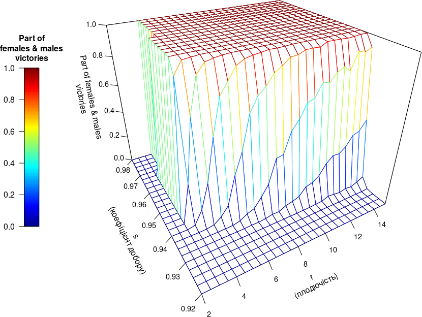
Next, it remains to build a diagram that will integrate the work of the Type III model as a whole. Now the Type III model as a whole can be presented.
# Sturtevant etc: ВПЛИВ ЧЕРГУВАННЯ ТИПІВ ДОБОРУ НА ХАРАКТЕР ВІДТВОРЕННЯ В ПОПУЛЯЦІЇ
# Модель III типа (аналіз впливу змінюваних початкових параметрів на розподіл імовірностей результатів)
# I. ENTRANCE — ВХІД:
# I.1. Initial script commands — початкові команди скрипту
# install.packages("plot3D")
library(plot3D)
# setwd("~/!_Courses/Sex_on_R") # Робоча директорія (лише на комп'ютері Д.Ш.!!!)
rm(list = ls()) # Очищення раніше збережених об'єктів в Environment
# set.seed(12345) # Використання певного варіанту вибору випадкових чисел
# I.2. Initial state of the system — початковий стан модельованої системи
al_0_N_fe <- 200 # Початкова чисельність самиць
al_0_N_ma <- 200 # Початкова чисельність самців
al_0_N_hp <- 0 # Початкова чисельність перехреснозапліднюваних гермафродитів
al_0_N_pg <- 200 # Початкова чисельність партеногенетиків
Genot <- c(0.11, 0.12, 0.12, 0.22) # Початковий розподіл генотипів: 11 = AA, 12 = Aa, 22 = aa
# I.3. Parameters — параметри
K <- 600 # Обмеження ємності середовища
# r <- 4 # ЗМІНЮВАНИЙ ПАРАМЕТР 1: Параметр Мальтуса, плодючість (розмір виводка)
# s <- 0.99 # ЗМІНЮВАНИЙ ПАРАМЕТР 2: Сила циклічно змінюваного негативного добору
# I.4. Experimental conditions — умови експерименту з моделлю
cycles <- 200 # Кількість робочих циклів моделі
iterat <- 100 # Кількість ітерацій
# I.5. The changeable parameters combinations — комбінації змінюваних параметрів
vector_r <- c(2, 2.5, 3, 3.5, 4, 4.5, 5, 5.5, 6, 6.5, 7, 7.5, 8, 8.5, 9, 9.5, 10, 10.5, 11, 11.5, 12, 12.5, 13, 13.5, 14, 14.5, 15)
vector_s <- c(0.92, 0.9225, 0.925, 0.9275, 0.93, 0.9325, 0.935, 0.9375, 0.94, 0.9425, 0.945, 0.9475, 0.95, 0.9525, 0.955, 0.9575, 0.96,  0.9625, 0.965, 0.9675, 0.97, 0.9725, 0.975, 0.9775, 0.98)
# II TRANSFORMATIONS SYSTEM CREATION — СТВОРЕННЯ СИСТЕМИ ПЕРЕТВОРЕНЬ:
# II.2. Parameters combinations mechanism — механізм комбінації змінюваних параметрів
ReproForms <- c("Females+Males", "Hermaphrodites", "Parthenogenetics")
Outcome <- array(NA, dim = c(length(vector_r), length(vector_s), length(ReproForms)), dimnames = list(vector_r, vector_s, ReproForms))
# Цикли, що перебирають досліджувані сполучення параметрів:
for (a in 1:length(vector_r)){ # Цикл, що змінює значення параметру Мальтуса
  r <- vector_r[a] # Змінюване значення чисельності популяції
  fe_O_FeMa <- r/2 # Кількість самиць у потомстві самиці (що була запліднена самцем)
  ma_O_FeMa <- r/2 # Кількість самців у потомстві самиці (що була запліднена самцем)
  hp_O_HpHp <- r # Кількість гермафродитів у потомстві гермафродита (що спарувався з іншим гермафродитом)
  pg_O_Pg <- r # Кількість партеногенетиків у потомстві партеногенетика (якому не треба з кимось паруватися)
  print(paste(a, "from", length(vector_r))) # Виводить у консоль кількість виконаних циклів вищого рівня
  for (b in 1:length(vector_s)){ # Цикл, що змінює максимальну тривалість життя
    s <- vector_s[b] # Змінюване значення сили добору
# II.3. Objects creation — створення об’єктів
rws <- c("Females_AA", "Females_Aa", "Females_aa", "Males_AA", "Males_Aa", "Males_aa", "Hermaph_AA", "Hermaph_Aa", "Hermaph_aa", "Parthen_AA", "Parthen_Aa", "Parthen_aa") # Рядки для масиву з підсумками
cls <- c(0:cycles) # Позначення стовпців для масиву з підсумками
itr <- 1:iterat # Створення вектору, куди будуть записані "імена" ітерацій
for (d in 1:iterat){First <- "Iteration_"; Second <- d;  itr[d] <- paste0(First, Second) } # Iterations names
Rez <- array(NA, dim = c(length(rws), length(cls), length(itr)), dimnames = list(rws, cls, itr)) # Створення тривимірного масиву для запису підсумків
Al_Pop <- rep(NA, al_0_N_fe + al_0_N_ma + al_0_N_hp + al_0_N_pg) # Створення вектору для початкової чисельності
# III. CALCULATIONS — РОЗРАХУНКИ:
# III.1. Higher level cycles running — запуск циклів вищого рівня
for (i in 1:iterat) { # Початок ітерації
# III.2. Initial composition creation — утворення початкового складу
if(al_0_N_fe>0) Al_Pop[1:al_0_N_fe] <- 1 # У файл для альфа-чисельності переносяться самиці...
if(al_0_N_ma>0) Al_Pop[(al_0_N_fe+1):(al_0_N_fe+al_0_N_ma)] <- 2 # ... самці...
if(al_0_N_hp>0) Al_Pop[(al_0_N_fe+al_0_N_ma+1):(al_0_N_fe+al_0_N_ma+al_0_N_hp)] <- 3 # ... гермафродити...
if(al_0_N_pg>0) Al_Pop[(al_0_N_fe+al_0_N_ma+al_0_N_hp+1):(al_0_N_fe+al_0_N_ma+al_0_N_hp+al_0_N_pg)] <- 4 # ... партеногенетики
Al_Pop <- Al_Pop + sample(Genot, al_0_N_fe + al_0_N_ma + al_0_N_hp + al_0_N_pg, replace=T) # Випадково визначаються генотипи усіх особин
# III.3. Main work cycle — основний робочий цикл
# III.3.a. Початок основного робочого циклу моделі
for (t in 1:cycles) {
  if(t>1) Al_Pop <- na.omit(Om_Pop) # В циклах крім першого Al_Pop - це Om_Pop попереднього циклу без NA
# III.3.b. Чисельність груп на початку циклу підраховується та переноситься у масив з результатами
  Rez["Females_AA", t, i] <- length(which(Al_Pop==1.11))
  Rez["Females_Aa", t, i] <- length(which(Al_Pop==1.12))
  Rez["Females_aa", t, i] <- length(which(Al_Pop==1.22))
  Rez["Males_AA", t, i] <- length(which(Al_Pop==2.11))
  Rez["Males_Aa", t, i] <- length(which(Al_Pop==2.12))
  Rez["Males_aa", t, i] <- length(which(Al_Pop==2.22))
  Rez["Hermaph_AA", t, i] <- length(which(Al_Pop==3.11))
  Rez["Hermaph_Aa", t, i] <- length(which(Al_Pop==3.12))
  Rez["Hermaph_aa", t, i] <- length(which(Al_Pop==3.22))
  Rez["Parthen_AA", t, i] <- length(which(Al_Pop==4.11))
  Rez["Parthen_Aa", t, i] <- length(which(Al_Pop==4.12))
  Rez["Parthen_aa", t, i] <- length(which(Al_Pop==4.22))
# III.3.d. Розрахунок бета-чисельності (альфа-чисельність + потомство), з ймовірнісним округленням
  be_N_Ma <- Rez["Males_AA", t, i] + Rez["Males_Aa", t, i] + Rez["Males_aa", t, i] # Загальна кількість самців
  if(be_N_Ma==0) { # Якщо самців нема, бета-чисельність дорівнює альфа-чисельності
    be_N_Fe_AA <- Rez["Females_AA", t, i]
    be_N_Fe_Aa <- Rez["Females_Aa", t, i]
    be_N_Fe_aa <- Rez["Females_aa", t, i]
    be_N_Ma_AA <- Rez["Males_AA", t, i]
    be_N_Ma_Aa <- Rez["Males_Aa", t, i]
    be_N_Ma_aa <- Rez["Males_aa", t, i]
    } else { # Якщо самці є, чисельність кожної форми розраховується залежно від схрещувань, де вона може утворюватися
  be_N_Fe_AA <- Rez["Females_AA", t, i] + floor(fe_O_FeMa * # Альфа чисельність + ймовірнісне округлення добутку плодючості та кількості схрещувань, де утворюється потрібний генотип
            (Rez["Females_AA", t, i] * Rez["Males_AA", t, i] / be_N_Ma +  # AA × AA  ⟶ AA
             Rez["Females_AA", t, i] * Rez["Males_Aa", t, i] / be_N_Ma / 2 + # AA × Aa  ⟶ AA : Aa
             Rez["Females_Aa", t, i] * Rez["Males_AA", t, i] / be_N_Ma / 2 + # Aa × AA  ⟶ AA : Aa
             Rez["Females_Aa", t, i] * Rez["Males_Aa", t, i] / be_N_Ma / 4) + runif(1)) # Aa × Aa  ⟶ AA : 2 Aa : aa
  be_N_Fe_Aa <- Rez["Females_Aa", t, i] + floor(fe_O_FeMa *
            (Rez["Females_AA", t, i] * Rez["Males_aa", t, i] / be_N_Ma + # AA × aa  ⟶ Aa
             Rez["Females_aa", t, i] * Rez["Males_AA", t, i] / be_N_Ma + # aa × AA  ⟶ Aa
             Rez["Females_AA", t, i] * Rez["Males_Aa", t, i] / be_N_Ma / 2 + # AA × Aa  ⟶ AA : Aa
             Rez["Females_Aa", t, i] * Rez["Males_AA", t, i] / be_N_Ma / 2 + # Aa × AA  ⟶ AA : Aa
             Rez["Females_Aa", t, i] * Rez["Males_Aa", t, i] / be_N_Ma / 2 + # Aa × Aa  ⟶ AA : 2 Aa : aa
             Rez["Females_Aa", t, i] * Rez["Males_aa", t, i] / be_N_Ma / 2 + # Aa × aa  ⟶ Aa : aa
             Rez["Females_aa", t, i] * Rez["Males_Aa", t, i] / be_N_Ma / 2) + runif(1)) # aa × Aa  ⟶ Aa : aa
  be_N_Fe_aa <- Rez["Females_aa", t, i] + floor(ma_O_FeMa *
            (Rez["Females_aa", t, i] * Rez["Males_aa", t, i] / be_N_Ma + # aa × aa  ⟶ aa
             Rez["Females_Aa", t, i] * Rez["Males_aa", t, i] / be_N_Ma / 2 + # Aa × aa  ⟶ Aa : aa
             Rez["Females_aa", t, i] * Rez["Males_Aa", t, i] / be_N_Ma / 2 + # aa × Aa  ⟶ Aa : aa
             Rez["Females_Aa", t, i] * Rez["Males_Aa", t, i] / be_N_Ma / 4) + runif(1)) # Aa × Aa  ⟶ AA : 2 Aa : aa
  be_N_Ma_AA <- Rez["Males_AA", t, i] + floor(ma_O_FeMa *
            (Rez["Females_AA", t, i] * Rez["Males_AA", t, i] / be_N_Ma + # AA × AA  ⟶ AA
             Rez["Females_AA", t, i] * Rez["Males_Aa", t, i] / be_N_Ma / 2 + # AA × Aa  ⟶ AA : Aa
             Rez["Females_Aa", t, i] * Rez["Males_AA", t, i] / be_N_Ma / 2 + # Aa × AA  ⟶ AA : Aa
             Rez["Females_Aa", t, i] * Rez["Males_Aa", t, i] / be_N_Ma / 4) + runif(1)) # Aa × Aa  ⟶ AA : 2 Aa : aa
  be_N_Ma_Aa <- Rez["Males_Aa", t, i] + floor(ma_O_FeMa *
            (Rez["Females_AA", t, i] * Rez["Males_aa", t, i] / be_N_Ma + # AA × aa  ⟶ Aa
             Rez["Females_aa", t, i] * Rez["Males_AA", t, i] / be_N_Ma + # aa × AA  ⟶ Aa
             Rez["Females_AA", t, i] * Rez["Males_Aa", t, i] / be_N_Ma / 2 + # AA × Aa  ⟶ AA : Aa
             Rez["Females_Aa", t, i] * Rez["Males_AA", t, i] / be_N_Ma / 2 + # Aa × AA  ⟶ AA : Aa
             Rez["Females_Aa", t, i] * Rez["Males_Aa", t, i] / be_N_Ma / 2 + # Aa × Aa  ⟶ AA : 2 Aa : aa
             Rez["Females_Aa", t, i] * Rez["Males_aa", t, i] / be_N_Ma / 2 + # Aa × aa  ⟶ Aa : aa
             Rez["Females_aa", t, i] * Rez["Males_Aa", t, i] / be_N_Ma / 2) + runif(1)) # aa × Aa  ⟶ Aa : aa
  be_N_Ma_aa <- Rez["Males_aa", t, i] + floor(ma_O_FeMa *
            (Rez["Females_aa", t, i] * Rez["Males_aa", t, i] / be_N_Ma + # AA × AA  ⟶ AA
             Rez["Females_Aa", t, i] * Rez["Males_aa", t, i] / be_N_Ma / 2 + # AA × Aa  ⟶ AA : Aa
             Rez["Females_aa", t, i] * Rez["Males_Aa", t, i] / be_N_Ma / 2 + # Aa × AA  ⟶ AA : Aa
             Rez["Females_Aa", t, i] * Rez["Males_Aa", t, i] / be_N_Ma / 4) + runif(1))  # Aa × Aa  ⟶ AA : 2 Aa : aa
           } # Закриття дужок підрахунку самиць та самців після else
  be_N_Hp <- Rez["Hermaph_AA", t, i] + Rez["Hermaph_Aa", t, i] + Rez["Hermaph_aa", t, i] # Загальна кількість гермафродитів
  if(be_N_Hp<2) { # Якщо гермафродитів менше за два, бета-чисельність дорівнює альфа-чисельності
     be_N_Hp_AA <- Rez["Hermaph_AA", t, i]
     be_N_Hp_Aa <- Rez["Hermaph_Aa", t, i]
     be_N_Hp_aa <- Rez["Hermaph_aa", t, i]
    } else { # Розраховується (з окремими позначеннями) чисельність різних за складом пар гермафродитів
      if(Rez["Hermaph_AA", t, i]>1) Pairs_Herms_AA_AA <- Rez["Hermaph_AA", t, i]*(Rez["Hermaph_AA", t, i]-1)/be_N_Hp else Pairs_Herms_AA_AA <- 0
      if(Rez["Hermaph_Aa", t, i]>1) Pairs_Herms_Aa_Aa <- Rez["Hermaph_Aa", t, i]*(Rez["Hermaph_Aa", t, i]-1)/be_N_Hp else Pairs_Herms_Aa_Aa <- 0
      if(Rez["Hermaph_aa", t, i]>1) Pairs_Herms_aa_aa <- Rez["Hermaph_aa", t, i]*(Rez["Hermaph_aa", t, i]-1)/be_N_Hp else Pairs_Herms_aa_aa <- 0
      Pairs_Herms_AA_Aa <- Rez["Hermaph_AA", t, i]*Rez["Hermaph_Aa", t, i]/be_N_Hp
      Pairs_Herms_AA_aa <- Rez["Hermaph_AA", t, i]*Rez["Hermaph_aa", t, i]/be_N_Hp
      Pairs_Herms_Aa_aa <- Rez["Hermaph_Aa", t, i]*Rez["Hermaph_aa", t, i]/be_N_Hp
      # А тепер - бета-чисельність різних генотипів залежно від кількості можливих схрещувань
      be_N_Hp_AA <- Rez["Hermaph_AA", t, i] + floor(hp_O_HpHp *
            (Pairs_Herms_AA_AA*2 + # AA × AA  ⟶ AA
             Pairs_Herms_AA_Aa + # AA × Aa  ⟶ AA : Aa
             Pairs_Herms_Aa_Aa/2) + runif(1)) # Aa × Aa  ⟶ AA : 2 Aa : aa
      be_N_Hp_Aa <- Rez["Hermaph_Aa", t, i] + floor(hp_O_HpHp *
            (Pairs_Herms_AA_Aa + # AA × Aa  ⟶ AA : Aa
             Pairs_Herms_AA_aa*2 + # AA × aa  ⟶ Aa
             Pairs_Herms_Aa_Aa + # Aa × Aa  ⟶ AA : 2 Aa : aa
             Pairs_Herms_Aa_aa) + runif(1))  # Aa × aa  ⟶ Aa : aa
      be_N_Hp_aa <- Rez["Hermaph_aa", t, i] + floor(hp_O_HpHp *
            (Pairs_Herms_Aa_aa + # AA × aa  ⟶ Aa
             Pairs_Herms_Aa_Aa/2 + # Aa × Aa  ⟶ AA : 2 Aa : aa
             Pairs_Herms_aa_aa*2) + runif(1)) # aa × aa  ⟶ aa
            } # Закриття дужок підрахунку гермафродитів після else
  be_N_Pg_AA <- Rez["Parthen_AA", t, i] + floor(pg_O_Pg * Rez["Parthen_AA", t, i] + runif(1)) # ...і партеногенетики
  be_N_Pg_Aa <- Rez["Parthen_Aa", t, i] + floor(pg_O_Pg * Rez["Parthen_Aa", t, i] + runif(1))
  be_N_Pg_aa <- Rez["Parthen_aa", t, i] + floor(pg_O_Pg * Rez["Parthen_aa", t, i] + runif(1))
  # III.3.e. Визначення добору для гомозигот та гетерозигот: залишок від поділу визначає, який йде добір
  if(t%%2==1) { # Якщо покоління непарне, то...
    v_homozygotes <- 1-s  # ...чисельність гомозигот скорочується, ...
    v_heterozygotes <- 1  # ...а чисельність гетерозигот лишається постійною
    } else {  # Якщо покоління парне, то...
      v_homozygotes <- 1  # ...чисельність гомозигот лишається постійною...
      v_heterozygotes <- 1-s}  # ...а чисельність гетерозигот скорочується
  # III.3.f. Вплив добору на кожну з груп (розрахунок гама-чисельностей)
  ga_N_Fe_AA <- floor(be_N_Fe_AA * v_homozygotes + runif(1)) # Додаток кожної бета-чисельності та...
  ga_N_Fe_Aa <- floor(be_N_Fe_Aa * v_heterozygotes + runif(1)) # ...життездатності у даному поколінні...
  ga_N_Fe_aa <- floor(be_N_Fe_aa * v_homozygotes + runif(1)) # ...зазнає ймовірнісного округлення:
  ga_N_Ma_AA <- floor(be_N_Ma_AA * v_homozygotes + runif(1)) # ...це і є гама-чисельність...
  ga_N_Ma_Aa <- floor(be_N_Ma_Aa * v_heterozygotes + runif(1)) # ...що розраховується...
  ga_N_Ma_aa <- floor(be_N_Ma_aa * v_homozygotes + runif(1)) # ...послідовно для усіх форм
  ga_N_Hp_AA <- floor(be_N_Hp_AA * v_homozygotes + runif(1))
  ga_N_Hp_Aa <- floor(be_N_Hp_Aa * v_heterozygotes + runif(1))
  ga_N_Hp_aa <- floor(be_N_Hp_aa * v_homozygotes + runif(1))
  ga_N_Pg_AA <- floor(be_N_Pg_AA * v_homozygotes + runif(1))
  ga_N_Pg_Aa <- floor(be_N_Pg_Aa * v_heterozygotes + runif(1))
  ga_N_Pg_aa <- floor(be_N_Pg_aa * v_homozygotes + runif(1))
  # III.3.g. Створення вектору з гама-складом популяції
  Ga_Pop <- c(rep(1.11, ga_N_Fe_AA), rep(1.12, ga_N_Fe_Aa), rep(1.22, ga_N_Fe_aa), rep(2.11, ga_N_Ma_AA), rep(2.12, ga_N_Ma_Aa), rep(2.22, ga_N_Ma_aa), rep(3.11, ga_N_Hp_AA), rep(3.12, ga_N_Hp_Aa), rep(3.22, ga_N_Hp_aa), rep(4.11, ga_N_Pg_AA), rep(4.12, ga_N_Pg_Aa), rep(4.22, ga_N_Pg_aa))
  # III.3.h. Створення вектора долі (Fate) і вектора жереба (Lot)
  if(length(Ga_Pop)>K) Fate <- rep(NA, length(Ga_Pop)) else Fate <- rep(NA, K) # Визначається довжина вектора долі
  Fate[1:K] <- 1 # В векторі долі стільки одиниць, скільки має вижити особин, але вони розташовані впорядковано
  Lot <- sample(Fate, length(Ga_Pop), replace = FALSE) # В векторі жереба одиниці та NA випадково переплутані
  # III.3.i. Вектор жереба визначає остаточний склад в циклі
  Om_Pop <- Ga_Pop * Lot # У векторі Om_Pop лишається K особин; загиблі особини - NA
  # III.3.j. Закінчення основного робочого циклу моделі і збереження результатів останнього циклу
  FM <- length(which(Om_Pop<3)) # Перевірка кількості трьох форм відтворення...
  Hp <- length(which(Om_Pop<4))-FM #...щоб у разі, коли залишається тільки одна...
  Pg <- length(which(Om_Pop<5))-Hp # ...перервати цикл та зекономити час
  if(FM==0 & Hp==0 | FM==0 & Pg==0 | Hp==0 & Pg==0) break # умова переривання даної ітерації
                     } # Основний робочий цикл моделі завершився
Rez["Females_AA", cycles+1, i] <- length(which(Om_Pop==1.11)) # Заповнення останнього стовпчику для результатів даної ітерації
Rez["Females_Aa", cycles+1, i] <- length(which(Om_Pop==1.12))
Rez["Females_aa", cycles+1, i] <- length(which(Om_Pop==1.22))
Rez["Males_AA", cycles+1, i] <- length(which(Om_Pop==2.11))
Rez["Males_Aa", cycles+1, i] <- length(which(Om_Pop==2.12))
Rez["Males_aa", cycles+1, i] <- length(which(Om_Pop==2.22))
Rez["Hermaph_AA", cycles+1, i] <- length(which(Om_Pop==3.11))
Rez["Hermaph_Aa", cycles+1, i] <- length(which(Om_Pop==3.12))
Rez["Hermaph_aa", cycles+1, i] <- length(which(Om_Pop==3.22))
Rez["Parthen_AA", cycles+1, i] <- length(which(Om_Pop==4.11))
Rez["Parthen_Aa", cycles+1, i] <- length(which(Om_Pop==4.12))
Rez["Parthen_aa", cycles+1, i] <- length(which(Om_Pop==4.22))
# III.4. Ending of higher level cycles — завершення циклів вищого рівня
                              } # Кінець циклу ітерацій
Outcome[a, b, "Females+Males"] <- sum(Rez[1:6, cycles+1, ])/(K*iterat)
Outcome[a, b, "Hermaphrodites"] <- sum(Rez[7:9, cycles+1, ])/(K*iterat)
Outcome[a, b, "Parthenogenetics"] <- sum(Rez[10:12, cycles+1, ])/(K*iterat)
                                    } # Кінець циклу, що змінює силу добору
                   } # Кінець циклу, що змінює значення параметру Мальтуса
## [1] "1 from 27"
## [1] ...
# IV. FINISHING — ЗАВЕРШЕННЯ:
# IV.3. Results viewing — перегляд підсумків
Outcome
## ...
# Results saving — збереження об’єктів з результатами
save(Outcome, file = "Outcome.RData")
# IV.4. Results visualization — візуалізація підсумків
persp3D(z = Outcome[, , "Females+Males"], x = vector_r, y = vector_s, theta = 330, phi = 30, # Побудова графіку
        xlab = "\nr\n(плодючість)", ylab = "\n\ns\n(коефіцієнт добору)", zlab = "\n\nPart of females & males\nvictories",
        expand = 0.8, facets = FALSE, scale = TRUE,  ticktype = "detailed",nticks = 6, cex.axis=0.9,
        clab = "Part of\nfemales & males\nvictories", colkey = list(side = 2, length = 0.5))