Biostatistics — 10. Topic 6. Comparison of distributions

6.1. Examples of Problems Requiring Distribution Comparison
Probably, distribution comparison is as frequent a task in biological research as value comparison. In this text, the topic of distribution comparison has been addressed at least three times.
First, an example of distribution comparison is the comparison of samples using Fisher's criterion, described in section 4.3 (see Fig. 4.3.1). This is a parametric comparison, as distributions in this case are compared by one parameter, based on the assumption that both samples have a normal distribution.
Second, the procedure for comparing distributions using Pearson's method is automatically invoked when comparing samples using the Kruskal-Wallis test, described in section 4.11 (see Fig. 4.11.3). This is quite logical: if we want to determine whether several samples belong to one or several general populations, we can use their comparison both by absolute values (comparison of means or medians) and by the nature of their distributions.
Third, we have already considered situations where it is necessary to check sample distributions for normality. This check makes sense in many cases when choosing whether parametric or non-parametric methods should be used. A simple method for such verification is described in section 5.2 (see Fig. 5.2.1).
As noted earlier (see section 1.5), not all traits are expressed as numbers from a continuous (metric) or discrete (meristic) numerical series. Many traits important for biological research are qualitative (polytomous or dichotomous), as well as ordinal in nature. To compare samples by such traits, distribution comparison is necessary. Let us give examples of several tasks requiring the use of methods discussed in this topic:
— do neighboring local populations differ in the frequencies of characteristic phenes (single qualitative external traits);
— do representatives of different sexes differ in susceptibility to a certain disease;
— does the use of a particular treatment method actually lead to more frequent patient recovery;
— do two (or more) qualitative traits vary dependently or independently in the studied population of objects.
Let us begin our consideration of distribution comparison methods with the use of Pearson's criterion to solve the last of these tasks.
6.2. Determining the Relationship of Qualitative Traits Using Crosstabulation
Let us turn to our Pelophylax_example.sta file. It examines 57 frogs belonging to 5 different genotypes and 2 different sexes. The distribution by sex and genotype of the studied frogs is not uniform: some combinations occur more frequently, others less so. Does the observed distribution reflect a relationship between sex and genotype? Can we assume that for some genotypes we statistically significantly more often encountered females, and for others—males?
To answer this question, we need to determine what distribution we would consider uniform. One in which all 10 (2×5) possible combinations of sex and genotype are represented with equal (or approximately equal) frequency? But, quite probably, some genotypes (for example, LLR) occur less frequently, and some (like RR) more often. How can we construct our study so that the different representation of genotypes and different representation of sexes in our sample does not prevent us from getting an answer to the question posed?
To answer this question, let us open the file Pelophylax_example.sta and follow the path Statistics / Basic Statistics and Tables / Tables and banners.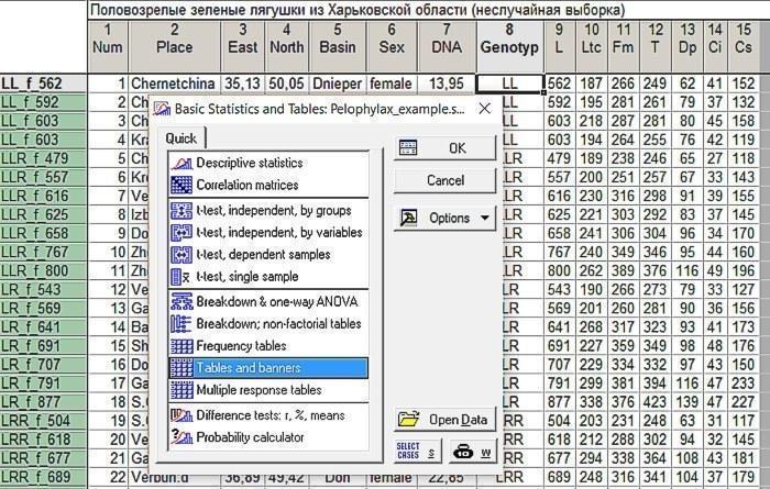

Fig. 6.2.1. A convenient dialog for comparing distributions is located here
We will go to the Crosstabulation Tables tab. There we will select the variables corresponding to sex and genotype.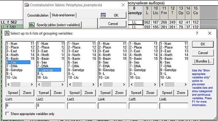

Fig. 6.2.2. Selecting the variables whose relationship needs to be analyzed
In the Crosstabulation Tables Results window, we will remove the checkmark from Highlight counts, which allows highlighting in red the values in those cells where relatively many observations fell (by default—10). We will put checkmarks in the Expected frequencies window, which outputs a separate window with expected frequencies (given the observed marginal sums), as well as in the Pearson & M-L Chi-square window, which invokes comparison of observed and expected frequencies using the method.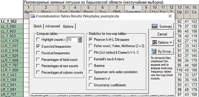

Fig. 6.2.3. Settings required for comparing expected and observed distributions
Clicking the Summary button, we will get two tables at once.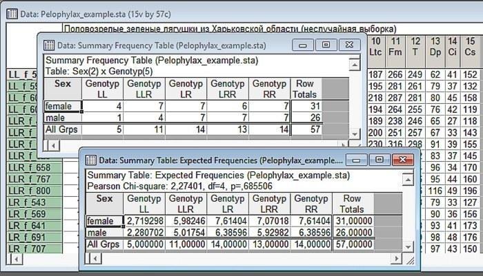

Fig. 6.2.4. Result of the analysis. Above—observed distribution, below—expected (given the same marginal sums). Make sure that the marginal sums (sums of elements in each row and each column) have not changed!
Interpretation of the first of the obtained tables is very simple. These are the observed frequencies of different combinations of the two selected variables. The variable selected first corresponds to the rows of this table, and the second variable corresponds to the columns. By the way, using this dialog one can also study the interrelationships of three or more variables, however, interpretation of such multi-entry tables turns out to be a non-trivial matter (try it and see for yourself!).
Marginal sums are calculated in the observed frequencies table. In our case, these are the total number of females and males, as well as individuals of different genotypes. Note: 5 frogs with the LL genotype were studied. The overall sex ratio in our sample is 31:26. If individuals with the LL genotype showed the same ratio, we could expect a ratio of approximately 2.7:2.8 in them. On the other hand, the overall genotype distribution in our sample is 5:11:14:13:14. If individuals were distributed uniformly, the same proportions would be observed both in females and males.
Thus, the table containing Expected Frequencies is constructed on the basis of empirically recorded marginal sums, on the basis of the assumption that the values of the considered variables are distributed independently of each other. Genotype distributions for different sexes correspond to the genotype distribution in the entire sample; sex distributions for different genotypes correspond to the sex distribution for the entire sample. This table gives the expected sex distribution in the case where the null hypothesis (postulating the absence of a relationship between variables) is true.
It remains for us to compare the observed and expected distributions. In the table this is done using the criterion (or goodness-of-fit test), proposed by Karl Pearson in 1900. Historians of science have expressed the opinion that the article in which Pearson proposed this criterion opened a new century in the history of statistics. Without going into detail, Pearson investigated how strongly the distribution of a sample can differ from the distribution of the general population from which it is obtained. The measure of difference between two distributions is calculated on the basis of the sum of squares of differences between observed and expected frequencies (in our case—the values in the cells of the two tables shown in the previous figure). Naturally, the "weight" of this measure of distribution difference depends on the number of degrees of freedom (the number of cells whose values can be changed independently). This measure of distribution difference is called . Probability distributions of have been constructed for different degrees of freedom; knowing the value of this quantity recorded in our comparison, we can determine the probability of its random occurrence (i.e., the probability of the null hypothesis).
Thus, in our comparison the calculated value of the criterion is 2.72, and the number of degrees of freedom df=4. Why exactly 4? Imagine that we have a table with given marginal frequencies. In one of the cells corresponding to females or males of the first genotype, we can enter any number not exceeding the number of representatives of this genotype (and the total number of representatives of this sex in the entire sample); by doing this we immediately determine the value of the second cell (it is calculated as the total number of representatives of this genotype minus the number of representatives of the first sex of this genotype). We can do the same with the second, third, and fourth genotypes. After that, the numbers of representatives of both sexes of the last, fifth genotype will already be rigidly determined (the number of females is calculated by subtracting the number of females of the first, second, third, and fourth genotypes from the total number of females). Thus, in a 2×5 table we can independently change 4 values, i.e., df=4.
As shown in the previous figure, the relationship between the considered variables in our example turned out to be non-significant (p=0.686; we have the case when Statistica does not put 0 before the decimal separator). Thus, the material in our study is represented unevenly, but we did not record a significant relationship between sex and genotype.
6.3. Comparing Distributions Using the Nonparametric Statistics Module
In the previous section, we took the recorded marginal frequencies (total number of males, females, as well as representatives of different genotypes) in our sample as given. We assumed that they reflect the different numbers of representatives of different sexes and different genotypes in the general population from which we obtained our sample. However, in some cases a different formulation of the question makes sense. Can we, on the basis of our sample, assume that different sexes and genotypes are distributed unevenly in the general population we are studying? For this we need to compare the recorded distribution with another one, where each cell contains the same number of individuals (it is easy to understand how to determine it: 57/10=5.7). For this we will have to create a file with such a distribution.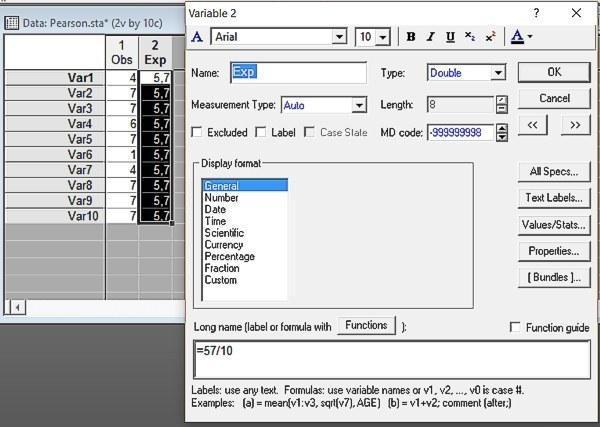

Fig. 6.3.1. The first column shows recorded frequencies, the second—expected frequencies in the case where the numbers of representatives of both sexes (as well as different genotypes) are equal
For the method of analysis we plan to use, it is important that the total size of both distributions is the same. In our case this condition is satisfied: we generated the expected distribution recalculated for the recorded number of individuals. The same method can be used to compare two empirical distributions, only in this case it is necessary to recalculate the larger one so that the number of observations in it corresponds to the smaller one.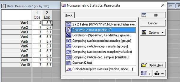

Fig. 6.3.2. The method we use belongs to the nonparametric ones
It remains to specify which distributions we are comparing and get the result.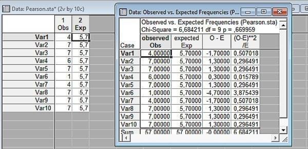

Fig. 6.3.3. Result of comparing empirical and calculated distributions. The difference is not significant
In the last figure we can see how the statistic is calculated. For each pair of cells (for each category of the distributions we are comparing) their difference is determined, which is squared and divided by the number of compared pairs. The sum of these quantities is the value of . Note: the value of in this case is higher than in the previous calculation, and the significance is lower. Why? Because the number of degrees of freedom is higher. In this case, knowing the total number of observations, we can independently change (within certain limits, of course) the values in 9 cells.
Thus, we did not find confirmation for the assumption that sex and genotypes of frogs are distributed unevenly (and in the previous section—that they are related to each other). On the basis of the data considered, we do not have sufficient reasons to reject the null hypothesis. An important addition is that for the considered problem it is known that the null hypothesis is incorrect. In the study area, frequencies of different genotypes are not equal; for some genotypes a sufficient predominance of males or females is observed quite often. However, these statements are made not on the basis of data contained in the file Pelophylax_example.sta, but taking into account other, significantly more representative studies.
Thus, in our case the null hypothesis is not rejected. As in all other cases, this does not mean that it is true.