
Ecology: The Biology of Interactions. 4.04. Exponential and Logistic Growth of Population Size
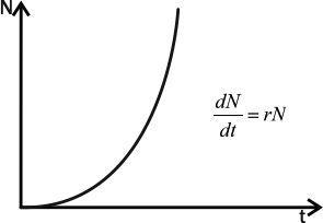
Population increase is proportional to population size; therefore, if growth is not limited by external factors, the population grows with acceleration. Its dynamics are described by the exponential population growth model. Naturally, exponential growth cannot continue forever. Sooner or later, resources are depleted, and growth slo...
Ukrainian language (latest version) / Russian language (no longer updated)
4.03. Demographic Tables, Pyramids, and Survival Curves
D. Shabanov, M. Kravchenko. Ecology: The Biology of Interactions Chapter 4. Population Ecology
4.05. Lotka-Volterra Model
4.04. Exponential and Logistic Growth of Population Size “In 1536, the Spanish adelantado Pedro de Mendoza, while founding Buenos Aires, brought 20 cows and 72 horses to the Argentine pampas. Three years later the settlement was burned by indigenous people, and the Spaniards abandoned it. Horses and cattle were left to themselves. They reproduced in the pampas, and by 1700 the cow population and horse population each reached one million head. Spanish sailors of the 16th and 17th centuries regularly introduced goats to oceanic islands to provide food in case of shipwreck. One such traveler, Juan Fernández, introduced a pair of goats to Pacific islands near the coast of Chile, islands later named after him. In 1704, when Alexander Selkirk (who served Daniel Defoe as a prototype for Robinson Crusoe) was left on these islands by his ship captain, the goat herd descended from that pair exceeded 10,000 and still exists” (O. Solbrig, D. Solbrig, 1982). Probably, the problem of describing population growth was first posed in “Liber abaci” by the Italian scholar Leonardo Fibonacci (1202). The book contains arithmetic and algebraic problems. One concerns rabbit reproduction dynamics: “A certain man places a pair of rabbits in a space enclosed on all sides by a high wall. How many pairs of rabbits are produced in one year from one pair, if each month a pair gives birth to another pair, and rabbits start reproducing from the second month after birth?” The solution is the series 1, 1, 2, 3, 5, 8, 13, 21, 34, 55 ... Thus, as Fibonacci already understood, population increment is proportional to population size; therefore, if population growth is not limited by external factors, it continuously accelerates. Let us describe this mathematically. Population increment is proportional to the number of individuals, i.e., ΔN ~ N, where N is population size and ΔN its change over a time interval. If the interval is infinitesimally small, we can write dN/dt = r × N, where dN/dt is change in population size (increment), and r is reproductive potential, a variable characterizing the ability of a population to increase in size. This equation is called the exponential population growth model (Fig. 4.4.1). [IMG_1] Fig. 4.4.1. Exponential growth The value r is sometimes called the Malthusian parameter. The English cleric Thomas Malthus was the first to note that human population grows in geometric progression. Familiarity with his work prompted both Charles Darwin and Alfred Wallace to infer that offspring of any organisms must be “thinned” by natural selection. As is easy to see, as time passes the population grows ever faster and soon tends toward infinity. Naturally, no habitat can withstand a population of infinite size. Nevertheless, there is a range of population-growth processes that within a certain time interval can be described by the exponential model. These are cases of unlimited growth, when a population colonizes an environment with excess free resources: cattle and horses colonizing pampas, flour beetles colonizing grain elevators, yeast colonizing a bottle of grape juice, etc. Naturally, exponential population growth cannot continue forever. Sooner or later resources are depleted and growth slows. What form will this slowing take? Practical ecology knows many variants: a sharp abundance outbreak followed by extinction after resource depletion, or gradual slowdown as abundance approaches a certain level. The simplest case is gradual braking. The simplest model describing such dynamics is the logistic model, proposed by the French mathematician P. Verhulst as early as 1845 (to describe growth of human population). In 1925, a similar pattern was rediscovered by the American ecologist R. Pearl, who assumed it was universal. The logistic model introduces variable K, the carrying capacity of the environment, i.e., equilibrium population size at which it consumes all available resources. Increment in the logistic model is described by dN/dt = r × N × (K - N)/K (Fig. 4.4.2). [IMG_2] Fig. 4.4.2. Logistic growth While N is small, increment is mainly controlled by factor r × N, and population growth accelerates. When N becomes high enough, factor (K - N)/K becomes dominant, and growth slows. When N = K, (K - N)/K = 0 and population growth stops. Despite its simplicity, the logistic equation satisfactorily describes many cases observed in nature and is still successfully used in mathematical ecology. Additional materials: Teaching model: Exponential growth Teaching model: Logistic growth 4.03. Demographic Tables, Pyramids, and Survival Curves
D. Shabanov, M. Kravchenko. Ecology: The Biology of Interactions Chapter 4. Population Ecology
4.05. Lotka-Volterra Model
4.05. Модель Лоткі-Вальтера