Lies, damned lies, and...

...statistics. Nowadays its use is almost an obligatory condition for carrying out scientific work in many fields, including zoology¹. It will not be much of a surprise if I say that statistics is used incorrectly more often than correctly. The reasons for this are varied, and we will try to discuss some of them.

One more introductory remark. Errors in the application of statistics are made by the most diverse specialists, including those with titles and - genuinely! - qualified ones. I will give examples from specific works by my colleagues. These people are no worse than others, and the reason I am citing them in particular is my acquaintance with them or my interest in their work. I do not want to violate their incognito. What is more, I cannot even name the object of their work. Zoology has a wonderful property, reflected by Boris Zakhoder in the fairy tale “The Whale and the Cat”. There, when an unexpected collision occurs (the whale and the cat swap places), a helicopter delivers to the deck of the whaling ship a group of responsible persons, among whom is “an academician for whales, an academician for cats”.

And in answer, at the whaling base
The helicopter lands straightaway.
In it are responsible persons
Who have flown in from the capital:
Doctors, professors,
A medical nurse,
An academician for whales,
An academician for cats,
With them seventy students,
Thirty-five correspondents,
Two editors with a proofreader,
A newsreel crew with a searchlight,
Young naturalists
And other specialists.

There are not enough posts in the academy for everyone, but people “in the know” understand that for whales it is N., and for cats it is either L. or M. In discussing specific stories, I will name certain objects. Well - those are not the real objects. Let us assume that any resemblance of the described circumstances to real works is coincidental.

So, let us proceed to examining the collection of difficulties that arise when using statistics in zoology.

Mistakes plus faith in “objectivity”

Let me start with a simple case. My colleague is a field man, better at handling a rifle than a computer. He had shot quite a number of... well, let us say, “hares”, and asked me to help count something about these hares. Which program does a Ukrainian or Russian zoologist turn to in such a situation? Often the Statistica package from StatSoft. This is a serious and expensive product. It is so expensive that, without discussing the specifics of domestic scientific and educational institutions, it is quite unclear how it could have gained such wide distribution². One of the reasons for its popularity is the variety of functions on offer and its high quality, but user conservatism also plays a role. About fifteen years ago Moscow and Kyiv zoologists used to pass each other floppy disks with the installer for the CSS statistical package, an earlier incarnation of Statistica. One way or another, this package has already become something of a semi-standard.

So then, I clarified what my “hare-ologist” colleague wanted, and made him a file. He sat a student down at the computer, who entered the measurement results into this file. Here is what happened next. I am hurrying to a meeting, and my colleague catches me in the corridor and drags me to the computer: “show me how to calculate this... correlation”. I show him: you need to call up such-and-such a window, select here the traits whose relationship you want to examine, and here the result will pop up. Having said this, I flee.

A week later another colleague of mine, an expert in English, catches me. The researcher of “hares” had asked him to translate an abstract intended for submission to the World Theriological³ Congress. The translator is puzzled: “Did you really calculate a significant negative correlation between body length and weight for him?”

I meet my “hare-ologist” colleague and ask: “You shot them yourself, did not you? Could you really not have noticed that the bigger the quarry, the lighter it is?” “You know, I was rather surprised myself that I had not noticed it. But those are my subjective impressions, and here we have a machine with all the objectivity inherent to it...”

I recalculate his results, look at the correlation. It is, naturally, positive. How the negative one came about there is now impossible to establish. It is a good thing at least the abstract had not managed to be sent off to the congress, there would have been quite some merriment there.

My colleague’s naivety laid bare a common trouble: we trust the results of calculations more than ourselves. Everyone makes mistakes, but sensible people organize their work process so that mistakes “surface” and can thereby be corrected. Here it is not out of place to mention one simple recipe.

With the help of statistics we look for one tendency or another reflected in the diversity of the material under study. But the mechanism with which we are endowed by nature (eyes and brain) also allows us to pick out fairly well the tendencies hidden within the diversity of the material. One simply needs to “feed” it information in a form convenient for perception. One of the good ways not to get confused in one’s criteria is to build graphs. When you see how the points are arranged, you can check any conclusion of yours. If some point “flies out” (is located apart from the main body), you can determine which case it is associated with. Sometimes it is convenient for this purpose to sort the rows in the data window by increasing value of the trait that interests you. And so that afterward you can return to the original order, it is convenient to make a column with the “correct” row numbers, sorting by which will return the table to its original state.

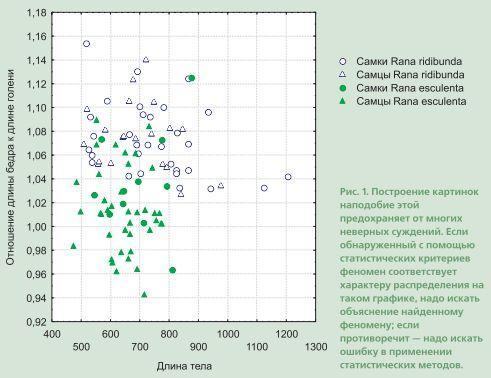
And one must never forget that the “machine” knows only what we have managed to tell it. And excessive trust in the results of calculations... Let me give the following example.

The program’s “default” settings

A defense of a doctoral dissertation is under way, by a major specialist in... well, let us say, “mice”. The author presents material from the whole of Eurasia: dozens of species, dozens of traits. Cluster analysis is used to determine similarity and difference between species. Independent cladograms (tree-like graphs reflecting the level of similarity within hierarchically subordinate groups) are built for females and males. The males’ cladogram looks quite ordinary, but the females’ looks strange (fig. 2). These cladograms are inserted into the autoabstract of the doctoral dissertation sent out to towns and villages and are shown at the defense.

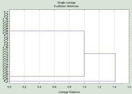
Fig. 2. Results of clustering the females of 30 “mouse” species by 50 traits (data conditional).

The dissertation author says that the variability of females and males follows different regularities, and draws attention to the fact that the females form two groups, within which they do not differ from one another. On this basis he manages to draw certain conclusions and hypotheses. Not one of the specialists present at the defense, or those who sent in reviews of the autoabstract, asks the elementary question: why, then, are they assigned to different species and even different groups of species, if by all the traits studied they are identical?

The box opens simply enough. The thing is that when carrying out cluster analysis in Statistica, one must decide what to do with the empty cells in the objects/traits table. By default, the corresponding module (fig. 3) has the “Casewise” option selected, which means that a trait for which at least one of the objects is undefined is discarded from consideration altogether. In our example this means that the specimens were classified using only two traits⁴, each of which can take only two values (for example, whether or not there are ear tufts).

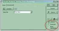
Fig. 3. The unfortunate little window in the cluster-analysis dialog

To compensate for the “holes” in the data, one must select the “Mean substitution” option. With this choice the missing value will be replaced by the mean for the entire set of objects and will have the least effect on the final result (of course, an even better solution is to determine all traits for all objects). Having chosen replacement by the mean value, we can obtain a tree resembling the one given for the males (fig. 4).

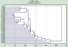
Fig. 4. Clustering of females again, using the same data as in fig. 2, only for the traits with missing data replacement by the mean value is switched on, instead of excluding the trait from the analysis.

Failure to understand the essence of the method

A prestigious scientific forum presented a work concerning the identification of morphotypes (groups of organisms united by similarity) in populations of animals which we will call “crows”. For many years I have been interested in the hypothetical possibility of correctly describing population diversity by singling out several morphotypes of individuals, so as then to compare populations by the frequencies of these types. And here I see a work in which this has been achieved...

The presence of several types in the “crow” population is illustrated by a picture analogous to the one shown in fig. 5. Here clustering by Ward’s method is used. This method builds clusters (groups) so that the resulting within-group variance is minimal. Unfortunately, the clusters that were identified when studying one sample did not correspond to the clusters that could be seen by similar methods in another.

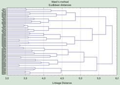
Fig. 5. Results of clustering 100 objects characterized by 100 random traits, using Ward’s method. One can see the formation of a number of groups at a similarity level of about 4 units

Having returned to the hotel, I built a table filled with noise (yes, the formula “=Rnd(1)” in a column header causes it to be filled with pseudo-random numbers from 0 to 1). Having clustered these random objects using the same methods, I obtained “morphotypes” grouped at roughly the same level of similarity as in the work on “crows” (fig. 5). What is characteristic is that this made no impression whatsoever on its author: “So what if groups are also singled out in random material? My material is not random!”

Singling out types only makes sense if they are separated from one another by a certain gap. If we analyze, using cluster-analysis methods, a set of objects belonging to types that are demarcated from one another, the clusters built in the course of the analysis will correspond to these types. But if there are no types in the structure of the material itself, the analysis will build clusters all the same: the work of its algorithms cannot end in anything else.

The magic of “significance”

The errors in the use of statistics described above were striking but fairly rare. Now, shuddering at my own audacity⁵, I must proceed to discuss an error that is the norm for a great many works, both in my own narrow specialty and in the study of related groups.

How does a taxonomist describe the diversity of organisms? Simplifying, one can say that he collects, in various regions, series of similar animals, compares them with one another, and decides whether they belong to the same form, to different subspecies, or to different species. New subspecies and species are described by indicating their differences from the old, previously known ones. In the old days this comparison was carried out mainly on the basis of the taxonomist’s intuition: his professional eye could (or could not) pick out the traits on the basis of which one decision or another was made. Nowadays it is customary to confirm one’s decision by statistical methods. How is this most often done?

Two series of objects are collected (for example, bleaks from the basin of river A and from the basin of river B), described by the maximum number of traits that allow them to be represented as numbers, and then compared across all these traits using Student’s and Fisher’s criteria (see box). The obedient Statistica will highlight in red those traits for which significant differences are found. Then we look at how many such traits are found and what status of difference they warrant. For example, in a domestic methodological compendium that is most authoritative for my branch of science, one of the classics indicated that two significant differences are too few to describe a subspecies, whereas three is just right.

Box

The expression “the samples were compared by Student-Fisher” carries a certain incorrectness within it. Even more often one encounters incorrect use of these methods.

Student’s criterion (the t-criterion) is the difference of the means of two samples, referred to the standard error of the difference of the sample means (which, in turn, depends on the level of variability of both samples). For each number of degrees of freedom (which depends on the sample sizes), it has been calculated with what probability the randomness of sample formation can lead to one value or another of the t-criterion. If the t-criterion for a given number of degrees of freedom exceeds a threshold value (for example, one arising by chance with a probability of 0.05), the difference between the samples can be considered significant.

The author of this most popular (unfortunately, not thanks to its merits, but owing to its simplicity) statistical method is the English chemist William Gosset, who worked for the Guinness brewing company. Under the company’s charter, its employees had no right to publish the results of research carried out as part of their official duties. Therefore Gosset published the results of his work in 1908 under the pseudonym Student.

It is fundamentally important that the t-criterion is defined only for the case when two samples with equal variances and normal distributions are being compared. If the variances in the samples differ, this fact can be shown using the F-criterion (the requirement of normality of distribution remains in force here). The F-criterion was proposed by the American statistician George Snedecor and named by him in honor of Sir Ronald Fisher, the English geneticist, creator of the analysis of variance. This criterion is a ratio of two variances. As with the t-criterion, the probability distribution of random deviations is known for it for various degrees of freedom.

Thus, the t-criterion allows one to assess the probability that the differences between the means of two samples reflect only random processes in their formation, while the F-criterion allows the same to be done with respect to the measure of their variability. Unfortunately, normality of distribution is the most important limitation on the applicability of these criteria.

Contrary to the prevailing opinion, normal distributions - are a rarity in biology. One of the classic examples of a “normal” distribution is the distribution of people by height. But look at the photograph: the distributions of men and women by height are different. In the photograph there are only healthy people, and no patients with hormonal imbalances. And just think what would happen if old people and children were added to this distribution!

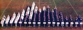
Normality of distribution arises when a quantity is affected by many unrelated weak factors. Biological diversity is usually affected by a whole bouquet of “strong” factors linked to one another by a bouquet of correlations. These factors are - sex, age, position in the population’s hierarchical structure, and much else. Unfortunately, in most cases it is better to say goodbye to “Student-Fisher”.

To describe new species, fortunately, something more than differences in metric traits is required (although apparently quite recently someone managed to describe a mass of new mollusk species almost exclusively on the basis of significant differences in shell shape). But to justify the existence of subspecies, the aforementioned considerations are used to the fullest.

Are they correct? Of course not. And the point is not only that the t- and F-criteria are applicable only to data with a normal distribution. The point is something else. “Student-Fisher” answers the question of what the probability is that two compared distributions of the same trait are drawn from one and the same general population, and that the differences between them are the result of chance in compiling the sample. If this probability (p) is below a certain level (for example, 0.05), we can take the risk and accept the hypothesis that the samples are drawn from different populations. This is what is called the significance of the differences. That is all. From this follow two consequences.

The first. When we compare bleaks from two different rivers, we already know from the very start that these are samples from different populations. The second. At a significance level of 0.05, a significant difference is one that arises no more often than in one case out of twenty. And if we compare samples across a hundred traits (or a hundred pairs of samples for one trait), the mathematical expectation of “significant” differences will amount to a whole five!

I take two groups of fifty objects each, characterize them by a hundred traits, filling the columns with noise. I compare using “Student-Fisher”. I get six “significant” differences, three of which fit into the very first screen (fig. 6). Well then, now one can analyze exactly which traits turned out to be significantly different, and draw profound conclusions on this basis about the specifics of the evolution of bleaks in the basins of the two rivers...

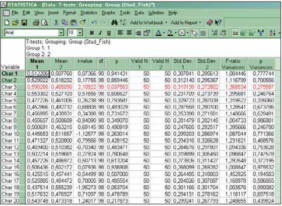
Fig. 6. Comparing two groups of objects by a set of random traits allows a certain
number of “significant” differences to be found.

Do my arguments seem primitive to you? Take any collection or journal with works similar in methodology and you will be able to find examples of such use of statistical methods yourself.

So what is to be done? For comparing samples by traits that do not follow a normal distribution, use non-parametric methods. For comparing several objects simultaneously, use analysis of variance. For comparing several traits at once, use multivariate criteria. For assessing the level of difference between various populations, calculate phenetic distances (numerical measures of how much two samples differ from one another). And use statistical methods more carefully.

Self-deception

We began the article with the peculiarities of working in the Statistica program. However, it is clear that the problem of using numerical methods in biology is broader than this program by itself. In the following example we are dealing with the mathematical modeling of evolution, but this work too can be regarded as connected with biometrics and statistics. Unlike the previous ones, this example cannot be made anonymous: it has already received far too much publicity. In describing it, I will refer to Darwin’s “Origin of Species”. To explain what Darwin has to do with it, we need to step aside a little.

I must confess that, having seriously “gotten hooked” on classical music, I categorically do not accept compilations like “The Best of Bach”. The authors of such selections take it upon themselves to touch up the classics. Great composers could sometimes compose something worthwhile, but, presumably for lack of taste, would insert hit-worthy melodies into tedious symphonies. Still, if one throws out everything unnecessary from an outdated piece, what remains may pass muster even for a modern, fastidious listener. Another sign of the times is the arranging of outdated music in a new manner. I have heard with my own ears complaints that Bach did not have an electric guitar at his disposal, what fine music he could have written⁶!

A similar tendency exists in the publication of the classics of science. An analogue of Bach with everything unnecessary thrown out and the remainder arranged for electric guitar might be Darwin’s “Origin of Species” as edited by A. V. Yablokov and B. M. Mednikov⁷. Those passages where Darwin was doubtful or cautiously feeling his way toward an idea have been thrown out by an unflinching hand. The remaining Darwinian text has been considerably “improved” with editorial comments and insertions. Since Darwin was not acquainted with Mednikov’s “Axioms of Biology”⁸, it was necessary to explain a few things to him. Among much else, a description of a machine experiment carried out by V. V. Menshutkin together with Mednikov himself has been added to “Origin of Species”, here there is no preserving the authors’ incognito... Although we are talking about a fairly old result, it is still often cited, so its analysis remains just as relevant.

The evolution of vertebrates was modeled. A “biosphere” was described in which a certain number of organisms could exist. A description of a vertebrate was set, in which a certain number of qualities (the presence/absence of various organs and properties) were listed. At the start, a creature of the amphioxus type was placed in the model biosphere, a primitive variant in which the adaptations of vertebrates exist only potentially. “Reproduction” was carried out by copying the organisms present in the biosphere. In the course of copying, errors, “mutations”, were possible. After each cycle of reproduction a surplus of organisms arose, and the program deleted the descriptions of the less well-adapted organisms, while sending the “genotypes” of the better-adapted ones on for further copying.

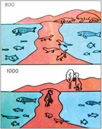
Fig. 7. Descriptions of two of the stages of machine evolution, “translated” into the language of images (Darwin (!), op. cit., p. 342)

As a result of this experiment it was possible to prove that the course of evolution is predetermined and inevitably leads to the emergence of intelligence. In the Menshutkin-Mednikov experiment, “amphioxi” gave rise to various “fish”, which had three pairs of paired fins, and then came out onto land in the form of six-legged creatures. As a result of the evolution of terrestrial life, creatures of the centaur type arose, organisms that moved on four legs, with front limbs free for labor. They had a large brain and a social life conducive to the development of intelligence.

Having reached this stage, the experimenters “rewound” the machine time and repopulated the land with four-legged creatures. Behold! Now the intelligence that arose in the course of evolution turned out to be bipedal. Thus it was possible to prove that there is a certain freedom in evolution, but on the whole its course is predetermined.

I believe that evolution is directional, but I am convinced of this not thanks to the Mednikov-Menshutkin experiment, but in spite of it. And the point is not that vertebrates could not have been six-legged (see box). The point is how, in this particular experiment, the fitness of the “organisms” was assessed.

Box

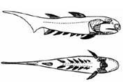
Terrestrial vertebrates are descendants of fish. Limbs arose from the paired fins of fish. The colonization of land by four-legged vertebrates is a consequence of the fact that fish have two pairs of paired fins: pectoral (front) and pelvic (rear). In the ancestors of fish, unpaired fins arose earlier, serving as a propulsor that ensured straight-line swimming during undulations of the body. The evolutionary formation of fish was linked to adaptation to predatory feeding and was accompanied by the acquisition of jaws (for seizing prey) and paired fins (rudders, ensuring turns). Paired fins formed from a lateral fold running along the body. As can be seen from the reconstruction of one of the most ancient fish, there were once more paired fins. In the fish shown in the figure, the intermediate fins have been transformed into spines. And as rudders, the most effective parts were the front and rear sections of what was once a single fin fold. Recall how it is easier to turn a boat around: by making a sideways stroke with the oar near the bow or near the stern, but not in the middle of the hull.

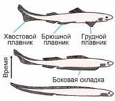
Can such interrelationships be taken into account in a model? In a complex one, yes. But if these interrelationships are understood, the problem is already practically solved. And to hope that the “machine” will itself “guess” such interrelationships is unforgivable naivety.

The book by Nobel laureate Friedrich von Hayek, devoted to attempts to manage the economy from a single center, is called “The Fatal Conceit”. No plan can foresee what is determined by a multitude of people in their specific market interactions. Even more fatal is the conceited belief that one can know in advance what natural selection will choose and what it will reject. A model biosphere capable of predicting this would have to be just as complex as the real one. But in the Menshutkin-Mednikov model there was only one way of separating successes from failures: to introduce an a priori assessment, in which whatever had triumphed in the course of actual earthly evolution was considered fit. The program was told that the most fit creature is an intelligent creature. Intelligence requires free limbs, a large brain, and social life. In other words, the model was given the final state and the way of reaching it (with the overcoming of random errors). Is anyone surprised that the model arrived exactly where it was directed to go from the very start?

It is interesting that the experimenters “switched off” evolution once an intelligent creature arose in it. Did they understand that the model’s further development would just be treading water? At the very least, they could have justified such a decision on the grounds that after the emergence of intelligence, biological evolution is displaced by social evolution. Either way, the experimenters convinced not only numerous readers but themselves as well of the predetermined nature of evolution. Darwinism is accused of circular logic: fitness is explained as the ability to survive, and survival is considered a consequence of fitness. Still, I think that Darwin, inclined as he was to cautious and thorough reflection, would not have fallen into the trap into which Menshutkin and Mednikov lured themselves. This, however, did not prevent their experiment from making it into an edition of one of the most important books in the history of biology (“The computer confirmed Darwin”).

What remains in the end? An example of self-deception. Unfortunately, other examples discussed in this article can be placed in the same category. However paradoxical it may seem, statistics is a widespread means of deceiving not only others, but oneself as well.

Have I mocked my own branch of science overmuch in this article? If I have mocked it, I hope I have not compromised it. Fortunately, when it comes to qualified specialists, their capacity for holistic perception of the material allows them to overcome the unfavorable consequences of the incorrect use of statistics. In fact, many statistical methods are designed precisely so that, amid the chaos of random deviations, one can pick out the deep causes of the observed variability showing through the interference. This lofty purpose of statistics compels us to treat it with respect, and this same purpose pushes us toward an uncritical faith in the results of “objective” proofs.

Returning to the title of the article, let us ask ourselves: which is better, a bold-faced lie or self-deception? I do not know. But with no connection whatsoever to statistics (and no call to deceive others rather than oneself), let me quote a principle that seems to me quite profound.

One of the difficulties in the formation of early Christianity was determining its relationship with Judaism, the traditional religion of the Jews. In the end Christianity distanced itself from Judaism, which contributed to its transformation into a world religion. This change even affected the interpretation of many Gospel events. In the canonical text of the Gospel of Luke, Jesus says, regarding the gathering of ears of grain on the Sabbath (that is, a violation of Old Testament rules): “The Son of man is Lord also of the sabbath.” There is also a known apocryphal variant of this Gospel, which contains another, most likely older (and possibly closer to the actual Jesus) variant⁹. Seeing a man working on the Sabbath, Jesus says: “Man, if indeed thou knowest what thou doest, thou art blessed; but if thou knowest not, thou art cursed, and a transgressor of the law.”