Ecology: the Biology of Interaction. VII-03. Arithmetic and Geometric Growth
What is distinctive about the growth of organism numbers as a result of reproduction? Can a growing population avert a Malthusian catastrophe? In this and the two preceding sections there is sufficient information to begin searching for answers to these questions using R. Believe us, this search may lead...
Appendices: Syllabus. Questions. References. Personalities. Glossary. R commands.
VII-3. Arithmetic and Geometric Growth
The universe is vast, but life is greater than it! ... The total quantity of matter in the universe remains constant, but life grows exponentially! The exponential is the mathematical devil.
Liu Cixin. The Dark Forest
VII-3.1. Two Playful Problems
Let us begin the discussion with two "mathematical" problems that should not be taken too seriously. Do not rush to find the answers; please read the first one and find the answer that seems correct to you. Then, without hurrying, find an answer that satisfies you for the second problem.
The first problem concerns hens. How many eggs will three hens lay in three days if one and a half hens lay one and a half eggs in one and a half days (Fig. VII-3.1)? Do not rush to read on — find the answer!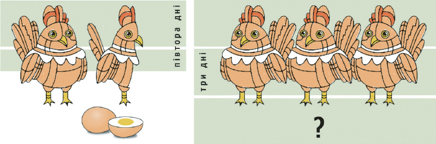
Fig. VII-3.1. The hen problem. One and a half hens lay one and a half eggs in one and a half days. How many eggs will three hens lay in three days?
It often seems that this problem is meaningless because it uses fractional values. This is not a problem; let us give an example of a perfectly serious use of fractional units when discussing reproduction. Thus, Ukrainian Wikipedia allows us to establish that the net reproduction rate (the number of daughters per woman who survive to their mother's age, at which the population size remains stable) in the modern world is close to 1.1. There must be 1.1 daughters per woman, and there is nothing paradoxical about this! Nobody expects the horrifying case of an unfortunate woman giving birth to one-tenth of a child. This value can be understood as follows: out of 10 women, 9 have one daughter each, and one has two.
Those who solve this hen problem correctly usually reason as follows. By how much did the number of hens increase? By how much did the laying time increase? Given a constant rate of reproduction, by how much should the result increase? What will it equal in that case?
Have you found the answer? The next problem concerns amoebae. Despite its hypothetical nature, it is based on entirely realistic figures. It uses the approximate maximum reproduction rate of Amoeba proteus and accounts for the average volume of its body. The simplification used in this problem is, of course, the assumption that under no circumstances would a given volume contain only amoebae, without the medium in which they exist.
Thus, we consider conditions under which amoebae and their offspring divide in half once per day; 28 days will suffice for a litre jar of amoebae to accumulate. How much time is required to obtain a litre jar from the offspring of two amoebae (Fig. VII-3.2)?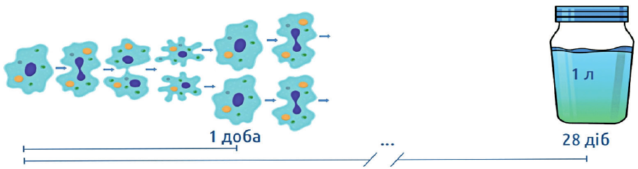
Fig. VII-3.2. The amoeba problem. An amoeba divides in half once per day; the next day each of the offspring also divides in half. As a result of cell division, the offspring of one amoeba fills a litre jar in 28 days. How long will it take the offspring of two amoebae to fill a litre jar?
Have you found the answer? Have you understood that the amoeba problem must be solved in a fundamentally different way from the hen problem (and it was precisely in order to complicate the solution of the amoeba problem that we started with the hen problem)? The point is that in the first case we are dealing with an arithmetic progression, and in the second with a geometric progression. An arithmetic progression is a sequence of numbers in which each successive term, starting from the second, differs from the preceding one by the same number — the common difference. If the common difference of an arithmetic progression is greater than 0, the progression is increasing. A geometric progression is a sequence of numbers whose first term is not zero, and the ratio of any element of the sequence to the preceding one is the same number — the common ratio. If the common ratio is greater than 1, the progression is increasing (variants with negative common ratios will not be considered here for simplicity).
The important point is that the number of organisms increases geometrically as a result of reproduction. In the first problem we are also dealing with reproduction, but we do not consider the addition of offspring to the number of breeders — we take a narrower time frame.
VII-3.2. The Sorrowful Discovery of Thomas Malthus
The study of organism reproduction was begun by Leonardo of Pisa (c. 1170 – c. 1250), better known as Fibonacci. At the beginning of the thirteenth century, in 1202, he published the "Book of Calculation" ("Liber abaci"), in which he examined a number of problems. Among them was a problem related to the reproduction of rabbits (which made rabbits a symbol of unrestrained reproduction and, presumably, the symbol of the erotic magazine Playboy and sexual permissiveness in general).
"Someone breeds rabbits in a space enclosed on all sides by a high wall. How many pairs of rabbits are born in one year from one pair if every month a pair of rabbits produces another pair, and rabbits begin to breed from the second month after their birth" (Fibonacci, 1202)
The solution to this problem is the so-called Fibonacci numbers: a sequence of numbers beginning with two ones (let us recall that the subject is pairs of rabbits, so one unit equals two breeders!), and each subsequent term of the sequence is the sum of the two preceding: 1, 1, 2, 3, 5, 8, 13, 21, 34, 55... This sequence of numbers has a number of remarkable properties in mathematics, but discussing them would take us far from the topic. Incidentally, have you understood that the answers to the problems posed at the beginning of this section are 6 and 27? Is it clear why?
The first person to clearly understand the full power of organism reproduction was the brilliant English clergyman, demographer, and economist Thomas Malthus (1766–1834). In his essay "An Essay on the Principle of Population" in 1798, he argued the following point. The size of a population grows in a geometric progression, while "the means of subsistence" (resources) grow arithmetically. The consequence of unrestrained growth must be an inevitable overpopulation catastrophe — the Malthusian catastrophe — in which a population growing faster than the "means of subsistence" will simply run out of food.
"I think I may fairly make two postulata. First, that food is necessary to the existence of man. Secondly, that the passion between the sexes is necessary and will remain nearly in its present state. <...> Assuming then my postulata as granted, I say that the power of population is indefinitely greater than the power in the earth to produce subsistence for man" (Thomas Malthus, 1798)
Malthus very intelligently discusses the consequences of this conclusion. He proposes late marriage, calendar contraception, abstinence, and assistance to the poor not in the form of food but support in organising their own enterprise. Incidentally, direct descendants of Malthus still live in England...
Communist ideologues accused Malthus of advocating war and the destruction of the poor — this is simply slander. To this day the widespread view persists that "Malthus has been refuted". This view rests on the fact that Malthus's reasoning quite understandably failed to account for two circumstances. First: the resources that sustain human existence grow not arithmetically but faster. Changes in farming practices cause intensification in the procurement of resources humans need. A hectare of arable land now yields far more food than in Malthus's time (at what cost — we discussed earlier in this textbook; primarily at the expense of vast quantities of fossil energy). Second: the rate of growth of the human population is declining, falling behind the geometric rate. This is understandable: in Malthus's time the demographic transition (see Section VI-7) had not yet occurred. Nevertheless, even from the quoted passage it is clear that Malthus did not regard his conclusions as independent of actual circumstances. In any case, he was the first to truly reflect on the influence of the reproductive power of living organisms on their resource availability.
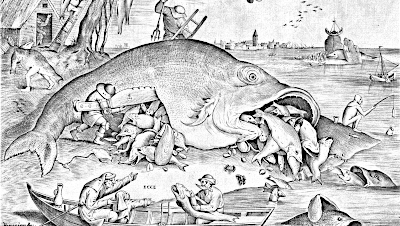
Incidentally, Malthus's work had unexpected consequences. The book was read by many people; the conclusions they drew from it corresponded to their level of understanding and reasoning. What matters for us is that at different times in the mid-nineteenth century this book was read by two British zoologists who had travelled on ships of the British Royal Navy, each of whose libraries contained a copy of Malthus's book. Both had observed differences in the fauna and flora of different continents and different islands. Both were searching for the cause of these differences. Both found a solution after reading Malthus's book (Fig. VII-3.3). The first of these researchers was Charles Darwin (1809–1882), the second was Alfred Wallace (1823–1913). Both understood that in nature all living creatures do not reproduce at the rate of which they are capable. It follows that the vast majority of individuals either never reach conditions suitable for reproduction or die before reaching maturity. Is survival and reproduction random? From this question springs the idea of natural selection!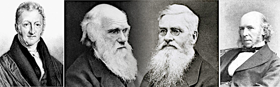
Fig. VII-3.3. The "fathers" of the concept of natural selection, four brilliant British scientists: Thomas Malthus (1766–1834), Charles Darwin (1809–1882), Alfred Wallace (1823–1913), Herbert Spencer (1820–1903)
VII-3.3. An Intellectual Challenge for Readers
From the information presented here it is clear that the problem of the relationship between arithmetic and geometric growth is very interesting. Let us formulate a question whose answer can be sought using simulation modelling with the tools described in Sections VII-2.1 and VII-2.2.
Task VII-3.1. Under what conditions does an increasing geometric progression fail to overtake an increasing arithmetic progression?
This question can be somewhat broadened.
Task VII-3.2. Under what conditions does a progression that is close to an increasing geometric progression but differs from it by a periodic decrease in the common ratio fail to overtake a progression that is close to an increasing arithmetic progression but differs from it by a periodic increase in the common difference?
The refinements introduced in Task VII-3.2 make it possible to account for the slowing of reproduction that may be associated with the demographic transition, and for the intensification of the economy.
An even broader way to formulate the problem posed is as follows.
Problem VII-3.1. Can a growing population avert a Malthusian catastrophe?
Dear readers! In this and the two preceding sections there is sufficient information to begin searching for answers to these questions using R. Believe us, this search may lead you to quite non-trivial and very important conclusions. Try to cover on your own that part of the path which is not prescribed here step by step. For example, you could create a model that compares arithmetic and geometric growth, similar to the one built in chunk VII-2.7. Most likely, in order to limit the range of data displayed in the graph, you will also need to use an if() condition that will terminate the simulation if geometric growth "wins the race" against arithmetic. There are many ways to construct a graph reflecting the modelling results; one of them is analogous to that shown in chunk VII-2.9.
Is this intellectual challenge sufficient to spur you to action?
VII-3.4. Result of Completing Task VII-3.1: The "Race" Between Arithmetic and Geometric Growth
Let us present the text of the script that accomplishes what was required in Task VII-3.1. First — the header and general matters. If you run this script on your computer, it may be useful to use the setwd() function to specify the path to your working directory. In this case, a commented-out reference to the working directory used by the author of this script is included. In your case, the directory address will most likely have a different format.
# Чанк VII-3.1
# «ПЕРЕГОНИ» АРИФМЕТИЧНОГО ТА ГЕОМЕТРИЧНОГО ЗРОСТАНЬ
rm(list = ls()) # Очищення Environment
# setwd("~/data/Eco_model") # Робоча директорія (виключно для D.Sh.!)
Both of the specified initial parameters relate simultaneously to both progressions – arithmetic and geometric.
# Чанк VII-3.2
# ЗАГАЛЬНІ ВХІДНІ ПАРАМЕТРИ ТА УМОВИ ЕКСПЕРИМЕНТУ
N1 <- 1 # Початкова чисельність популяції (однакова для обох прогресій)
t <- 1000 # Тривалість експерименту (максимальна кількість кроків)
We create a vector where an arithmetic progression will be built. We start with the parameter a, which is only needed for its construction. Let's pay attention to one circumstance. Further, we will not break down comments in chunks into separate lines (this way they will be better perceived). However, this may lead to the fact that these long lines will be broken in random places, including within words, where line breaks are not possible. For RStudio to correctly display such lines, check the option Code/Soft Wrap Long Lines in the menu.
# Чанк VII-3.3
# АРИФМЕТИЧНЕ ЗРОСТАННЯ:
# Вхідний параметр, що визначає прогресію
a <- 1000 # Доданок арифметичної прогресії. Показує, яка величина додається до кожного попереднього значення арифметичної прогресії
# Створення об'єкта для запису результатів
arithm <- rep(NA, t) # Створення пустого вектора для запису арифметичної прогресії
# Початковий стан
arithm[1] <- N1 # Перенесення першого значення з загальних умов
We do the same for a geometric progression
# Чанк VII-3.4
# ГЕОМЕТРИЧНЕ ЗРОСТАННЯ:
# Вхідний параметр, що визначає прогресію
q <- 1.1 # Знаменник геометричної прогресії. Показує, на яку величину множиться кожне попереднє значення геометричної прогресії
# Створення об'єкта для запису результатів
geom <- rep(NA, t) # Створення пустого вектора для запису геометричної прогресії
# Початковий стан
geom[1] <- N1 # Перенесення першого значення з загальних умов
The working cycle is ready to start. If the geometric progression does not catch up with the arithmetic one, the cycle will stop when the cycle counter i reaches the value t. If the geometric progression catches up with the arithmetic one, the cycle will stop due to the condition built into it. In this case, it is useful to see at which i this happened.
# Чанк VII-3.5
# РОБОЧИЙ ЦИКЛ
for(i in 2:t) {arithm[i] <- arithm[i-1] + a
               geom[i] <- geom[i-1] * q
               if(geom[i]>arithm[i]) break} # Цикл перераховує значення лічильника циклу i у вказаних межах. У фігурних дужках і послідовних рядках (або в одному рядку через точку з комою) — команди, що виконуються для кожного значення i. Команда if() перевіряє, чи перегнала геометрична прогресія арифметичну, та, у разі, якщо перегнала, зупиняє цикл for командою break
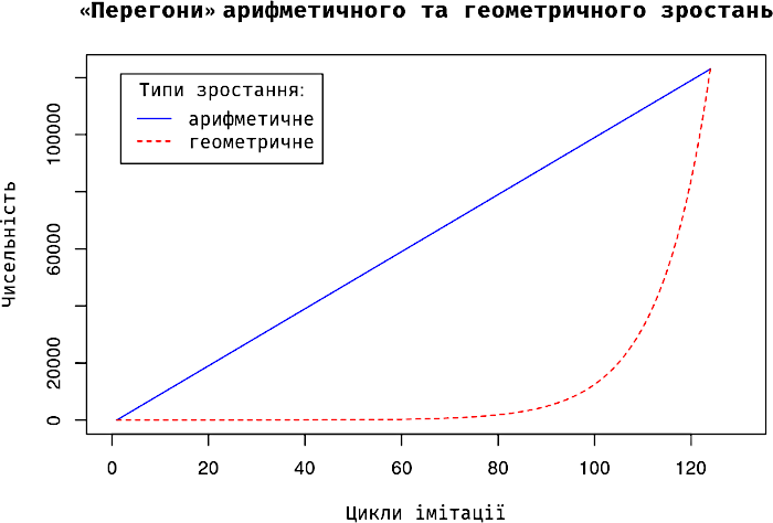
i # Виводить значення i, на якому зупинився цикл for; це — момент "перемоги" геометричного зростання над арифметичним
## [1] 124The diagram remains to be added.
# Чанк VII-3.6
# ПОБУДОВА ГРАФІКА
plot(arithm,  # Будуємо найпростіший графік; вказуємо джерело даних
     xlim=c(0, i*1.05), # Діапазон значень осі абсцисс (осі x)
     type="l", lty=1, col="blue", # ...тип, характер та колір лінії
     main="«Перегони» арифметичного та геометричного зростань", # Заголовок
     xlab="Цикли імітації", ylab="Чисельність") # Підписи осей
lines(geom, type="l", , lty=2, col="red") # Додаємо на графік ще одну лінію
legend("topleft", inset=.05, title="Типи зростання:", c("арифметичне", "геометричне"), lty=c(1, 2), col=c("blue", "red")) # Додаємо легенду (розшифровку)
Both of the specified initial parameters apply simultaneously to both progressions — arithmetic and geometric alike.
We create a vector in which the arithmetic progression will be built. We begin with the parameter a, which is needed only for its construction. Let us draw attention to one circumstance. Hereafter we will not split comments within chunks into separate lines (they will be easier to read that way). However, this may result in long lines breaking at random positions, including in the middle of words where line breaks are not possible. To have RStudio correctly wrap such lines, tick the option Code/Soft Wrap Long Lines in the menu.
We do the same for the geometric progression.
Everything is ready to launch the working loop. If the geometric progression does not catch up with the arithmetic, the loop will terminate when the loop counter i reaches the value t. If the geometric progression catches up with the arithmetic, the loop will be stopped by the condition built into it. In the latter case it is useful to see at which value of i this occurred.
It remains to add the diagram.
# Чанк VII-3.7
# АРИФМЕТИЧНЕ, ПРИСКОРЕНЕ АРИФМЕТИЧНЕ, ГЕОМЕТРИЧНЕ ТА ЗАГАЛЬМОВАНЕ ГЕОМЕТРИЧНЕ ЗРОСТАННЯ
rm(list = ls()) # Очистка Environment
# setwd("~/data/Eco_model") # Робоча директорія (виключно для D.Sh.!)
The model we are creating has a significantly larger number of parameters than the previous one. The text of the previous model was organized as follows: first, an arithmetic progression was defined, then a geometric one, and only in the working cycle were the calculations related to both progressions combined. It is better to organize this model differently, building blocks according to calculation stages. And the first solution is to gather parameters and conditions into one block.
# Чанк VII-3.8
# ЗАГАЛЬНІ ВХІДНІ ПАРАМЕТРИ ТА УМОВИ ЕКСПЕРИМЕНТУ
a <- 1000 # Доданок арифметичної прогресії; щоб прогресія зростала, має бути >0
q <- 2 # Знаменник геометричної прогресії; щоб прогресія зростала, має бути >1
period <- 10 # Проміжок часу між змінами показників модифікованих зростань
add_a <- 100 # Показник прискорення модифікованого арифметичного зростання
decr_q <- 2 # Показник гальмування модифікованого геометричного зростання
N1 <- 1 # Початкова чисельність популяції (однакова для обох прогресій)
t <- 1000 # Тривалість експерименту (максимальна кількість кроків)
All progressions will be collected into vectors organized in the same way.
# Чанк VII-3.9
# СТВОРЕННЯ ОБʼЄКТІВ:
arithm <- rep(NA, t) # Арифметичне зростання
geom <- rep(NA, t) # Геометричне зростання
m_arithm <- rep(NA, t) # Модифіковане арифметичне зростання
m_geom <- rep(NA, t) # Модифіковане геометричне зростання
In addition to transferring the initial value to the created vectors, we will need two things. To change the parameters of the modified progressions, while leaving the parameters of the standard arithmetic and geometric progressions unchanged, we need to set new values. Initially, the modified parameters are equal to the unmodified ones, and then they can change. These changes will occur periodically; to count these periods, we need to start a separate counter.
# Чанк VII-3.10
# ПОЧАТКОВИЙ СТАН:
arithm[1] <- N1; geom[1] <- N1; m_arithm[1] <- N1; m_geom[1] <- N1 # Усі прогресії починаються з того самого значення
m_a <- a; m_q <- q # Модифіковані прогресії починаються з тих самих показників, що й не модифіковані
p <- 0 # Лічильник періоду змін показників
Main part. Working cycle. In it, the next values of all progressions should be calculated. It is logical to calculate the values of the modified progressions after checking whether their parameters should be recalculated. We have set the initial value of the parameter change period counter; its value increases by one in each cycle. If the value reaches the required level, the counter returns to its initial value, and the parameters of the modified progressions are recalculated.
# Чанк VII-3.11
# РОБОЧИЙ ЦИКЛ
for(i in 2:t) {
  arithm[i] <- arithm[i-1]+a
  geom[i] <- geom[i-1]*q
  p <- p+1
  if (p==period) {m_a <- m_a+add_a
                  m_q <- m_q - (m_q-1)/decr_q # Принципово важлива формула. Можливі інші рішення!!!
                  p <- 0 }
  m_arithm[i] <- m_arithm[i-1]+m_a
  m_geom[i] <- m_geom[i-1]*m_q
  if(m_geom[i]>m_arithm[i]) break}
i # Виводить значення i, на якому зупинився цикл for; це - момент "перемоги" загальмованого геометричного зростання над прискореним арифметичним — мальтузіанська катастрофа. Якщо її не буде, кількість циклів визначатиме t
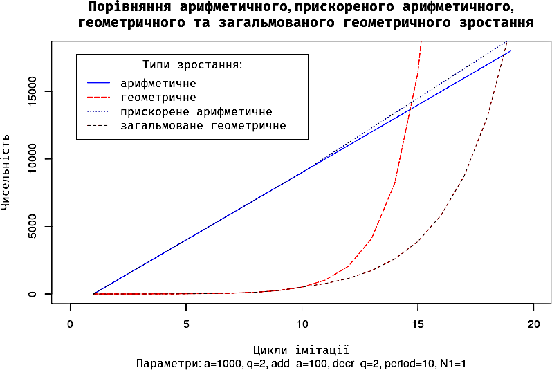
## [1] 19In the given example, the adjustment of the common ratio of the geometric progression occurs as follows: periodically, a certain part of the difference between the current value and one is subtracted from this common ratio. This is far from the only possible value. It is interesting to try other options! We are dealing with a model that depends on a sufficiently large number of parameters. The result of the model's operation will most likely be a graph. To compare different cases more easily, it is convenient to display the parameter values used in the calculations on the graph. We will generate an object that we will then display as a subtitle on the diagram we are building. For this, we will use the paste0() command: it combines the arguments enclosed in parentheses separated by commas. Note: text fragments are enclosed in quotes, and variables are indicated without quotes; in the latter case, the numerical value of the variable will be output.
# Чанк VII-3.12
# ПОБУДОВА ГРАФІКА
Param <- paste0("Параметри: a=", a, ", q=", q, ", add_a=", add_a, ", decr_q=", decr_q, ", period=", period, ", N1=", N1) # Підпис зі значеннями усіх параметрів, що будуть вказані на графіку
Let's see what we got.
# Чанк VII-3.13
Param
## [1] "Параметри: a=1000, q=2, add_a=100, decr_q=2, period=10, N1=1"All that remains is to build the diagram. For simplicity, we will display all four lines on the graph.
# Чанк VII-3.14
plot(arithm,  # Перша лінія
     xlim=c(0, i*1.05), # Діапазон значень осі абсцис (осі x)
     type="l", lty=1, col="blue", # ...тип, характер та колір лінії
     main="Порівняння арифметичного, прискореного арифметичного,\n геометричного та загальмованого геометричного зростання", # Заголовок
     sub = Param,
     xlab="Цикли імітації", ylab="Чисельність") # Підписи осей
lines(geom, type="l", , lty=5, col="red") # Додаємо ще лінії
lines(m_arithm, type="l", , lty=3, col="blue4")
lines(m_geom, type="l", , lty=2, col="brown4")
legend("topleft", inset=.05, title="Типи зростання:", c("арифметичне", "геометричне", "прискорене арифметичне", "загальмоване геометричне"), lty=c(1, 5, 3, 2), col=c("blue", "red", "blue4", "brown4")) # Легенда