Ecology: Biology of Interaction. VII-01. First Steps in Using RStudio

Section VII (additional). Simulation modelling in R in the ecology course
VII-1. First Steps in Using RStudio
I heard — I forgot.
I saw — I remembered.
I did — I understood.
(Attributed to Confucius)
VII-1.1. The R Language
The history of R began with the S language, developed by Bell Labs — an American company that played a key role in the development of software. It was a language designed for statistical computations (which explains the letter S), named by analogy with the programming language C. Over time, an S+ version also appeared. Both S and S+ were commercial and rather expensive products. In due course, activists of the GNU project took an interest in this language. The GNU project (GNU's Not UNIX) was launched in 1983 by Richard Stallman. This American programmer left the university so that an operating system similar to Unix (a modular operating system based on ideas developed at Bell Labs) would not belong to any organisation. Stallman's initiative led to the emergence of the free software developer movement. In 1991, Linus Torvalds began work on the kernel of an operating system version that came to be called Linux. Both Linux and other free software products are, in our view, the most striking examples of achievements of human cooperation.
Naturally, in time two GNU activists decided to create a free analogue of S+ within the framework of this project. Staff members of the Statistics Department of the University of Auckland (in New Zealand), Ross Ihaka and Robert Gentleman, began work on solving this problem in 1992. In 1993 the first experimental implementation of this free statistical programming language appeared. By analogy with S, this language also received a name consisting of a single letter — the first letter of its creators' first names. Over time, the R community grew enormously.
R is a free, open-source product. It is a programming language for solving problems in the field of statistics and modelling, as well as an open-source environment for computation and graphics. R is distributed as source code as well as a compiled (translated from programming language to machine code) program. R is available for Linux (a “related” operating system, another result of the development of Bell Labs approaches in the GNU project), Windows, and macOS. In general, this language is a large-scale result of the altruistic activity of an enormous community of intellectuals from around the globe, with a special role for representatives of the New Zealand school of statistics. The centre around which this community is organised is the website r-project.org. Over time, popular innovations spread within the R community. One can work with “bare” R, or use various shells. The most widely used shell for R is RStudio. The scientific director of RStudio, a professor of statistics at the University of Auckland (and a biologist by his first degree) Hadley Wickham, has significantly influenced the development of the R language. In particular, he is the author of the concept of tidy data and a number of popular packages that are part of the tidyverse suite. The most popular of these packages is ggplot2, which has in effect become one of the standards of scientific graphics. The tidy data concept is not fundamentally new; many of its components have long been known (for example, the approach of “observations in rows, characteristics or attributes in columns” and many other requirements, which are, among other things, set out in the “canon for constructing a table for primary data collection”). Nevertheless, its integration into the practice of routine computations in R is an important matter.
For our course, all three persons mentioned above can be considered “founding fathers” (Fig. VII-1.1), since we will be using R through the RStudio shell and may apply parts of the tidyverse suite.

Fig. VII-1.1. “Gurus” of R: Ross Ihaka and Robert Gentleman (source), Hadley Wickham (source)
R is a high-level, object-oriented, interpreted, scripting programming language. The high-level nature of this language is related to the fact that its constructs are oriented towards the human mind rather than the computer processor (though this mind must work logically, consistently, and unambiguously). R is object-oriented in that it contains descriptions of individual objects with certain attributes. Objects can belong to two categories: data objects, intended for storing data, and function objects, which perform certain transformations on other objects. The object with which a function has worked does not itself change; to preserve the results of a function's operation, these results must be converted into a new object, or the old object replaced by the new one via a separate command. To understand the advantage of R's interpretability, one should note that programming languages can be compiled or interpreted. Programs in compiled languages are “translated” into the language of codes controlling the processor as a whole. Programs in interpreted languages are converted line by line into codes using a certain interpreter, or “translator.” Scripting languages are characterised by the use of certain sequences of actions utilising existing objects and functions. Because R is an interpreted scripting language, a program written in R — a script (a chain of commands) — can be executed step by step or in part. This is very convenient for debugging such a program when something has not worked on the first attempt (i.e., in the typical case). An R script can be modified at any point. To repeat a previously executed sequence of operations in R, it suffices to modify the script and run it again.
Are the tasks that can be solved using R unique to this language? No. The same results can be obtained using various languages. Thus, an alternative to R can be Python — another free programming language. However, one should understand that Python has a broader field of application (and is therefore more popular), but is less convenient for solving tasks typical of R. For a long time, R has remained the “champion” in terms of convenience, power, and flexibility for solving a certain category of tasks. The tasks we will consider in this tutorial belong to this category.
Like it or not, to use R one must overcome a certain entry threshold. A typical situation is one where a person who has had no prior R experience (and, worse, who has had experience with programs organised in a fundamentally different way) tries to solve some task in R. In the first steps, nothing will be comprehensible! The playful approach, which requires intuitively transparent operational logic, does not work in a programming environment that demands unambiguity. Quite often this leads to frustration with R and a return to less sophisticated tools. On the other hand, when dealing with a specialist who uses this language, one can conclude that they have learned to overcome obstacles and, when necessary, can manage their own frustration.
It should be noted that typical work with R can consist of step-by-step overcoming of difficulties: there is something to be done; one searches for information, makes attempts, fails, looks for the causes of failures, overcomes them step by step, optimises the script, corrects errors, reaches a dead end, finds a way out… and ultimately derives satisfaction from solving the problem.
…one of the authors of this tutorial was on an internship at one of the world's leading universities with a specialist who had made significant progress in applying R. The intern wished to use the master's time as efficiently as possible. A few days before the substantive meeting, the intern tried to solve the problem independently and immediately encountered difficulties. Clearly, the necessary transformations were possible, but how? Intuitively obvious approaches led to program halts and strange messages… The intern did not want to spend shared working time on what could be found online. He searched for solutions to analogous problems in Google, found analogies, tried to apply them, and failed time and again. In such a situation it is hard not to swear out loud; it is clear that neither R nor the authors of the advice that could not be applied are to blame for anything, but swearing somehow alleviates the feeling of failure… Nevertheless, after spending several hours searching and making fruitless attempts, it was eventually possible to advance one step. Before the first shared session with the master, it had been possible to take several such steps. And then the moment came when the intern explained what help was needed. “I have no idea how to do this,” said the guru: “We need to search.” The specialist went to Google; it should be noted that he formulated his queries such that he obtained results more quickly. The first attempts to apply what was found were unsuccessful; the master received error messages from R and swore in response. Since both the master and the intern belonged to the same culture, the expletives they used in case of failure were more or less similar… Nevertheless, the guru was able to take the needed step quite quickly, then another. The specialist's qualification was manifested not in the fact that he knew the answer to non-trivial questions in advance (or even in the fact that he swore more effectively), but in the fact that through trial and error, using the collective wisdom of the network, he advanced much faster than a novice. In the end, the model that was being built during that internship was completed. It immediately became clear that it was not optimal; the script had to be corrected. During experiments with the model it turned out that one of the assumptions made during its construction was unfortunate; the model had to be rewritten… Dear students! If during your work with R you feel like fools, and R at some moment seems to be a means of tormenting you, do not worry: these are typical experiences. What matters is that they do not stop you. If your efforts continue, you will prevail, and thanks to the efforts expended, the sense of your victory will be especially acute.
VII-1.2. Installing R and RStudio
In this section, the simulation modelling capabilities provided by the R language will be used. To work with this language we will use the shell program RStudio. The simplest way to use them is to install them on your computer. First, R should be installed, and only then RStudio. The R installer is freely available here, and the RStudio installer — here. Choose the versions intended for your operating system!
If, for example, you are working on a device (smartphone, tablet) running Android, you will have to use an online service, for example, this one (Fig. VII-1.2).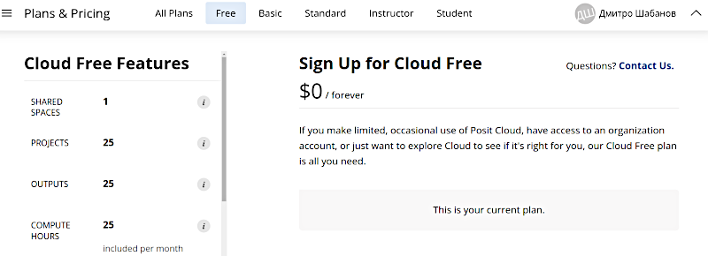

Fig. VII-1.2. The Posit Cloud service offers cloud access to R and RStudio. You can register here and choose free access (which has significant limitations). Unfortunately, this solution is in many respects not the most convenient.
In what follows we will illustrate the discussion using the example of the installed RStudio.
VII-1.3. RStudio Windows
After the RStudio installer has finished its work, it will most likely not launch anything. You will need to find this program yourself, either in the Start menu or among the list of installed programs. Launch it! If you have done everything correctly (you did not forget that RStudio needed to be installed after R?), you will see the following (Fig. VII-1.3).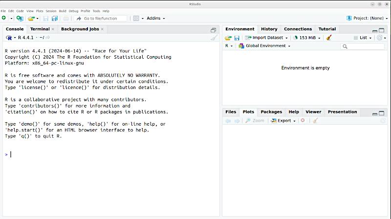

Fig. VII-1.3. RStudio has just been launched for the first time.
In Fig. VII-01.3 you can see that the RStudio window is divided into separate panels. One more panel is absent. Let us invoke it. Select the File menu, then New File, and then — R Script. Now the RStudio window is divided into four panels (Fig. VII-1.4).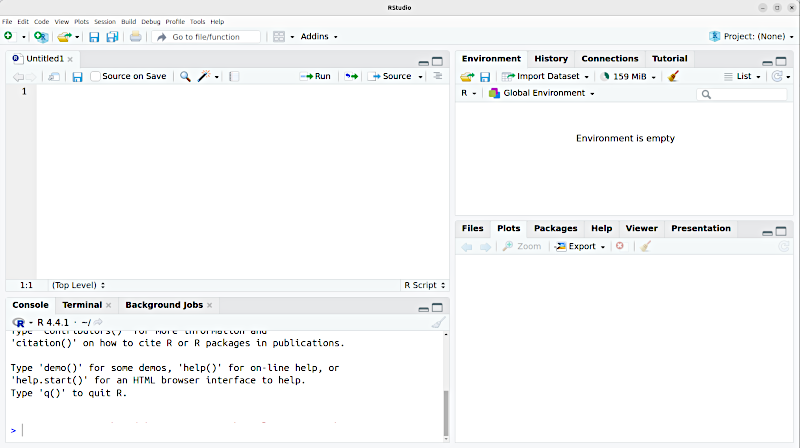

Fig. VII-1.4. The script editor has been invoked.
As stated above, R is a scripting language, i.e. an R program is a script, a chain of commands that can be executed in full or in part, and to any point of which changes can be made. In Fig. VII-1.4 we see the script editor; it is located in the upper left panel of the RStudio window, and it has opened the script Untitled1  (since it has not yet been saved). Let us enter some command in this editor, for example, type “2*2”.
We can now execute this command. To execute a single line of the script, we must place the cursor in that line and press either the Run button or the two keyboard keys simultaneously: Ctrl+Enter (Fig. VII-1.5).
We will immediately note two more ways to run R commands. A certain number of lines can be selected with the cursor and Run pressed. Furthermore, when the script has already been saved (more on this later), the Source button can be pressed; in this case R will once again save the file with the script and execute it in full.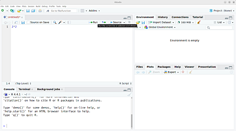

Fig. VII-1.5. One way to execute the command contained in a line of the script is to place the cursor in that line (or select it) and press the Run button.
The command has been executed (Fig. VII-1.6). The result appeared in the console (the lower left panel of the RStudio screen). First, the console shows the command that R executed; this command is shown after the symbol >. Then comes a line with the results. The elements of this line are numbered; the number of the element that begins the line is shown in square brackets. Since the line with the response to the command “2*2” consists of one element, this is the number we see in the console before the result. 
Why does this panel of RStudio have the name “console”? Once, in the era of large computing machines, input and output devices were mounted on special supports or brackets. In architecture, a console is a support with one end fixed and the other free. Since that time, “console” in programming has designated a device (physical or software) for data input and output.
Incidentally, the command “2*2” or any other could have been entered directly in the console — try doing this. However, for creating programs (and a simulation model in R is precisely a program), scripts must be used. Get in the habit of entering commands in the script editor!
Let us complicate the task. Let us create a certain object and assign it a certain value. Type in the script editor “vect <- 1:10”. This command has three elements. First, vect is the name of the object. It will be created because the assignment operator follows it: <-. If this operator is applied to an object that already exists, it will overwrite its contents. If this object did not yet exist, it will be created. And the third element is the content of the created object. Here the : function is used, which creates a sequence of integers from the first, which is specified before its designator (the colon), to the last, which is specified after the colon.
This text is intended for a first acquaintance with R, and therefore it will not contain a complete list of either the types of objects used in this language or the types of data that are possible here. Nevertheless, let us note that the basic object in R is a vector — a sequence of elements. And so, the : function creates precisely a vector (which is why we gave this object the name we did). 
The command we have used does not require anything to be displayed in the console; there only a report on which command was executed will appear. But the result of execution (the new object) appeared in the upper right panel of the RStudio screen — in the Environment window. Listed here are the objects with which R is working during the current session (Fig. VII-1.6).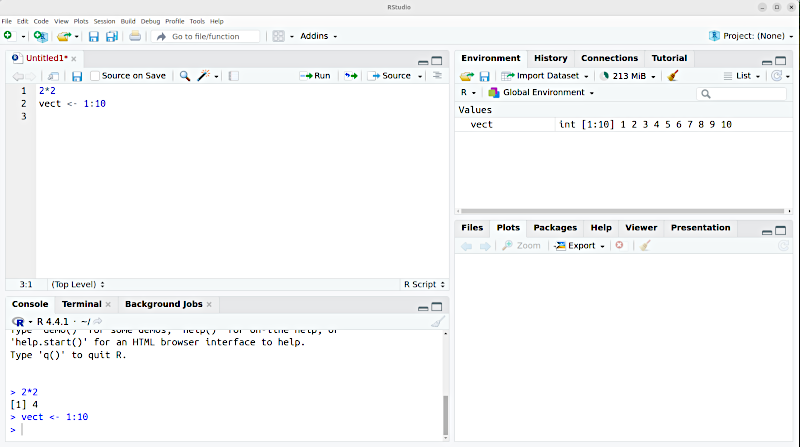

Fig. VII-1.6. In the console — a report on the execution of two commands. In Environment — the created object, a vector of integers from 1 to 10.
To understand what is located in the lower right panel of the RStudio window, let us execute the command plot(vect). The plot() function constructs a diagram, the format of which depends on the characteristics of the object it operates on. That it is indeed a function is indicated, among other things, by the parentheses appended to its name. Inside these parentheses, arguments must be specified — parts of the command that indicate what this function will operate on and how it will operate (Fig. VII-1.6). The : function, with which you have just become acquainted, is in this sense atypical; it is used without parentheses, simply connecting the arguments between which it is placed.
The plot() function should construct a diagram based on the object vect. When we enter the name of this object, RStudio will offer us a hint in a small pop-up window, a hint tooltip (Fig. VII-1.7). The hint with a list of suggestions for automatic completion of function or object names can be invoked (by beginning to type a name) deliberately; to do this press Tab or Ctrl+Space.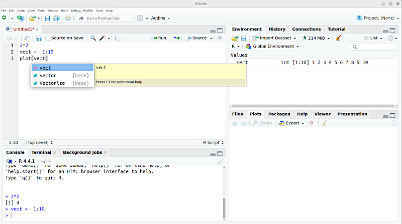

Fig. VII-1.7. A hint — a pop-up tooltip in RStudio.
We have not specified any additional arguments in the command plot(vect). Bear in mind: the plot() function, as you will see subsequently, can have a very large number of arguments! As long as the task this function is to perform has not been specified in greater detail, it will create the simplest variant of the diagram provided by default. The result will be shown in the lower right panel of the RStudio window, on the Plots tab (Fig. VII-1.8).
By the way, Fig. VII-1.8 illustrates another important feature of R: a script can be commented. Everything located in a given line after the # symbol (the “hash”) will be ignored during script execution. This is text intended not for R, but for the human reader. RStudio highlights such comments in green. One can comment out (i.e., exclude from execution) part of a line that follows the “hash,” an entire line, or even several lines. The fact is that sometimes, when working with a script, it is useful to comment out a certain part of it (for example, to provide the model with different sets of initial parameters, uncommenting the one needed and commenting out the unnecessary ones). In such cases, the required set of lines should be selected and Ctrl+Shift+C pressed. This command will comment out uncommented lines and uncomment commented ones.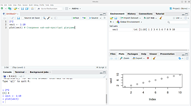 

Fig. VII-1.8. A diagram has appeared on the Plots tab.
Let us use RStudio screenshots to show one more feature of working with this program. When saving a script in which symbols other than the typical Latin character set were used, RStudio will ask you to specify which code page (the correspondence between the codes stored in the file and the characters) should be used. Fig. VII-1.9 was created in Ubuntu, one of the versions of the Linux operating system; in this system UTF-8 is used as the default code page.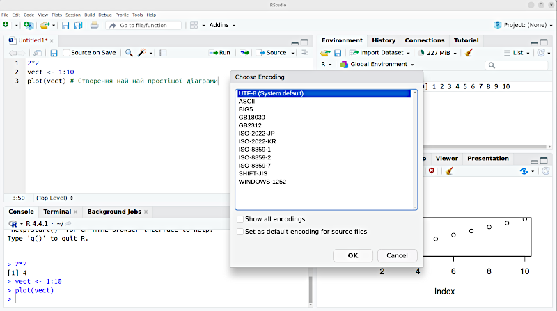

Fig. VII-1.9. Choosing a code page when saving a script.
Up to this point we have used a very uneconomical way of demonstrating how R works — providing screenshots. Going forward we will use a more sophisticated approach and make use of the tools of the R Markdown text markup language.