Creation of Worlds — 06. Analytical insertions in the simulation model

6. Analytical Inserts in Simulation Models
6.1. Modeling the Interaction of Individual Individuals with Individual Resource Units
In the previous model, we described a mechanism that reduces the number of a group of individuals that differ in competitiveness to the quantity ωN, corresponding to a certain resource availability (V). It should be noted that in one important respect, the mechanism we used differs from what we can observe in reality. If resources are sufficient for 100 individuals, and the population consists of 100 individuals, 100 will likely remain. But if the population consists of 200 individuals? A significant portion of them will die, but ultimately, probably not 100 will remain, but a smaller number of individuals (since those individuals who were destined to die will have consumed a certain amount of resource, and less will remain for those who survive). And if 10,000 individuals compete for the amount of resources that can support 100? In reality, it would be good if any of them survive...
How to reflect these patterns in a simulation model? To do this, it is inevitable to transition to modeling the interaction of individual individuals with individual resource units. The point is that in order to account for the reduction in the amount of resource as a result of its consumption by those individuals who will only partially satisfy their needs and then die, we must somehow consider how the portions of what each individual must receive in order to remain alive are distributed.
Thus, we consider a set of individuals (a simpler variant — of groups of identical individuals) that consume a certain number of resource units — one can, if desired, speak of "frogs" catching "flies". What is important is that the probability of consuming a resource unit by different individuals may differ. Strictly speaking, resource units can also differ ("flies" can be "large" or "small", for example).
The probability of a particular individual consuming a particular resource unit depends on the composition of all individuals competing for the resource. Depending on the number of individuals and their ability to acquire the resource, this probability may differ, and determining it in advance is very difficult. Fortunately, it is much easier to determine the ratio of probabilities of acquiring a particular resource unit for two different individuals. Not knowing what population conditions these individuals will find themselves in, we can nevertheless assume that one of them has, for example, twice the chance of acquiring a resource unit as the other. We will denote such relative probability as q (from English quota). In this case, jqg is the relative probability of acquiring a j-th category resource unit for the g-th individual. A single value of jqg by itself has no meaning; what is important is the ratio of these values for different individuals or different categories of individuals.
How to transition from the set of jqg to the set of jpg, i.e., the probabilities of acquiring a j-th category resource unit for the g-th individual in a particular population environment? As follows: jpg=jqg/Σ(jqg).
Let us solve a relatively simple task: simulate the distribution of 500 resource units, of which 300 belong to category 1 (say, "small flies"), and 200 belong to category 2 (say, "large flies"), among 8 individuals ("frogs"). Let us denote the quantities of these resource categories as follows: 1V=300, 2V=200; capital letters indicate that we are estimating the total number of resource units.
Let us set the relative probabilities of acquiring these resource units for all individuals (Fig. 6.1). You see that these relative probabilities are set as whole numbers. This is not necessary but is convenient and provides a simple way to understand their essence. Since Σ(1qg)=19, we can consider that we have specified quotas for the distribution of 19 "small flies" among 8 "frogs". The probabilities 1pg must be proportional to these quotas. It is in this way that we will calculate all the probabilities we need.
By the way, the input parameters in the model we began constructing in Fig. 6.1 are the relative probabilities, jqg, while the calculations use the absolute probabilities, jpg, which are determined on the basis of the relative ones. Unique names (thanks to which it will be easier to understand the formulas) will, of course, be given to the absolute probabilities, jpg. The format of such names can be seen in the left part of Fig. 6.1.
Our further calculations will be significantly simplified if we also calculate cumulative probabilities for each resource category: besides 1p1, we will also calculate 1p1-2=1p1+1p2, 1p1-3=1p1+1p2+1p3, and so on. It is clear that 1p1-8=2p1-8=1. The cells with these values will also need special names; we will give them according to a somewhat different pattern (Fig. 6.1, right part).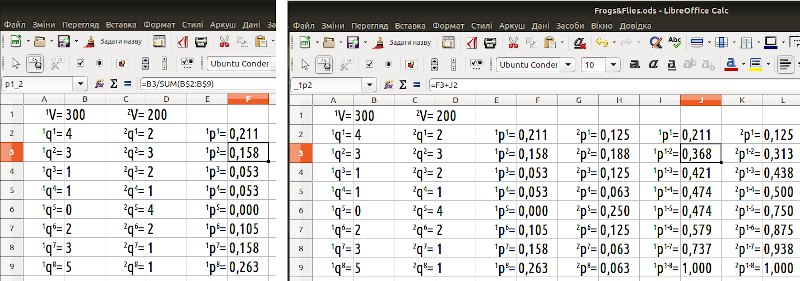

Fig. 6.1. In the two parts of this figure, one can see what names the probabilities jpg and cumulative probabilities jp1-nreceive, as well as the formulas by which they are calculated
To simulate the distribution of 500 resource units, we will need 500 random numbers uniformly distributed between 0 and 1. Let us create a block of such numbers. The author of this course usually places random numbers in cells with a yellow background, as done in Fig. 6.2. Depending on the value of the random number and the distribution of cumulative probabilities, we will determine which individual receives each resource unit. We will do this in a block of cells located under the block with random numbers. It remains only to count how many of each resource unit each individual receives using the COUNTIF function (Fig. 6.2)...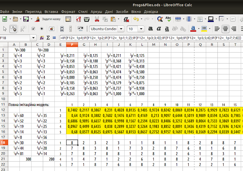

Fig. 6.2. Note the formula bar. This formula determines which individual will receive a particular resource unit. We divide the range from 0 to 1 according to the values of cumulative probabilities jp1-nand determine in which part the random number falls
Let us present the formula visible in Fig. 6.2 more clearly:
=IF(F12<_1p4;IF(F12<_1p2;IF(F12<_1p1;1;2);IF(F12<_1p3;3;4));IF(F12<_1p6;IF(F12<_1p5;5;6);IF(F12<_1p7;7;8))).
We used a "three-story" formula. The first IF determines whether the resource unit falls into the first half of the distribution or the second; in both cases, the next IF formula determines which quarter the resource unit falls into; at the end, the next IF establishes which individual will receive this unit.
Although the model we described was built fairly quickly, it is quite "heavy," primarily because to model the fate of 500 resource units, we needed 500 random numbers. If the model is large enough, it will not only take a long time to perform each calculation; unfortunately, the probability of errors will also increase significantly. Remember that in this case we are using spreadsheets not for their intended purpose!
Can these calculations be simplified somehow?
6.2. Functions for Modeling Binomial Distribution
Binomial distribution is the distribution of a certain number of successes from a certain number of trials with a given probability of success for each trial. To understand which functions are available in LO Calc for working with this distribution, let us consider a simple example.
We roll a die (a cube with six faces) six times (or roll 6 dice at once). How many times can a one appear? From zero to 6. Each time, the probability of rolling a one (as with any other face, in the case of a perfect die) is 1/6. Presumably, the probabilities that in the experiment with 6 die rolls, a one appears 0, 1, or, say, 6 times are different. What are they?
Let us use the function =BINOM.DIST(number of successes;number of trials;probability of success;parameter). If the parameter in the formula equals 0, the function determines the probability of the specified number of successes; if the parameter equals 1, the function determines the probability that the number of successes will be no more than the specified. For example, the formula =BINOM.DIST(0;6;1/6;1) determines the probability that a one (with a probability of 1/6 for each trial) will appear once, and =BINOM.DIST(0;6;1/6;1) — that it will appear no more than once (i.e., either zero times or once).
Figure 6.3 shows both formulas and values simultaneously. In the second row, the BINOM.DIST formula is applied with parameter 0, and in the third row — with parameter 1. Note: the value in cell B3 equals the sum of the values in cells A2 and B2. Thus, with a probability of about 73%, a one will appear no more than once. To see both the formulas and the values calculated from them in Fig. 6.3, one can use a method we have not yet used: enable formula viewing using the command "View / Show Formula".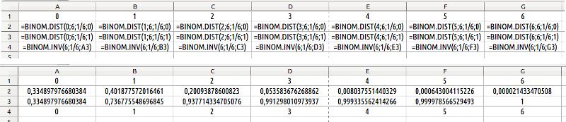

Fig. 6.3. Formulas for working with binomial distribution. The upper part of the figure demonstrates the formulas, the lower part — the corresponding values
In the fourth row, the function BINOM.INV is used, which calculates the inverse, i.e., inverted binomial distribution. In this function, the order of arguments is somewhat different from the previous one we considered: =BINOM.INV(number of trials;probability of success;probability of result). One can consider that this function answers the following question: given the number of trials and the probability of success in each trial, no more than what number of successes will be observed with the specified probability. The result of calculations by this function is rounded to integer values.
What result will the use of the formula =BINOM.INV(6;1/6;B3), located in cell B3 in Fig. 6.3, give? From 6 trials and a probability of success in each trial of 1/6, no more than how many successes will be observed with the probability specified in cell B3? This function outputs 1 — no more than one success will occur in 73% of attempts of six die rolls...
If you understand how the BINOM.INV function works, you are ready to apply it in our model.
6.3. How Many "Flies" Will Each "Frog" Get According to Binomial Distribution?
We have established that the BINOM.INV function answers the question: given the number of trials and the probability of success in each trial, no more than what number of successes will be observed with the specified probability. The number of trials is given by the number of resource units (by the way, in the model and formulas they have the names _1V and _2V). The probabilities of successes in each trial are the jpgvalues we calculated (as can be seen in Fig. 6.1, they are denoted as p1_1, p1_2 ... p1_8, p2_1 ... p2_8). The specified probability of the number of successes, not less than which we will observe, will be determined by a random number. It remains for us to place the cells with random numbers and with calculations using the BINOM.INV function on the LO Calc sheet (Fig. 6.4).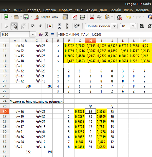

Fig. 6.4. The model built on binomial distribution requires much fewer calculations and less space on the sheet (here it is spent uneconomically; for example, cells B26:B33 simply duplicate H26:H33 for more convenient comparison with the results of the "full" modeling)
Thus, instead of 500 random numbers and 500 "three-story" formulas, we only needed 16 of each. In fact, instead of applying simulation (step by step deciding the fate of each resource unit), we applied an analytical formula. In the first section, we compared analytical and simulation models. In previous models, we saw the advantages of simulation modeling — it can be carried out even without having a complete understanding of the processes being modeled, the simulation model can be step-by-step improved, and, in general, it is more flexible than an analytical one. But, as this example demonstrates, significant advantages also exist in analytical models. In cases where the task can be reduced to finding the solution of some known equation, analytical models turn out to be much more economical and efficient.
Well, we can combine the advantages of both simulation and analytical modeling in our work!
There is also an important difference, which is also easy to see in Fig. 6.4. The "full" model distributed 300 units of the first type of resources and 200 of the second. This will be the number of these units when recalculating the obtained distribution. The analytical insert we applied distributed 322 units of the first type of resources and 197 of the second; upon recalculation, this number will change time and time again. The point is that in the first case, we tracked 500 individual units; in the second — we obtained 18 random estimates. Of course, in the case of multiple repetitions of calculations using the second model, we will register that the "frogs" received on average 300 units of the first type of resources and 200 of the second. In the first model, 1V=300and 2V=200— the exact quantity of resources, in the second — the mathematical expectation, the mean value in the case of multiple observations.
And which is correct? There is no unambiguous answer; everything depends on which aspects of reality are more important when building our models. However, when it comes to ecological systems, the quantity of available resources is better estimated as a certain mathematical expectation (a value whose exact value can be influenced by random factors), rather than as a precisely set quantity. The statement that, for example, the "frogs" of a certain "pond" "eat" 500 "flies" per day operates with an approximate estimate of the number of these "flies," since no one will count them individually. From this point of view, the probabilistic result we obtained using binomial distribution is more adequate. However, it is easy to imagine tasks where one will need to calculate exactly a certain number of resource units. For example, if we are interested in how 8 "frogs" will be distributed among the "snakes" that will eat them, we will probably need to investigate the fate of exactly 8 individuals.
At the end of the previous section, we compared the distributions generated by two different models — deterministic and probabilistic. For this, we used an iteration counter. We can use such a counter in this case as well. We need to add a counter to the model where calculations are carried out in two different ways, calculate and save a certain number of distributions obtained by both methods, combine these distributions into two groups, and compare them with each other.
Task. Compare the distributions of 500 resource units using the two models discussed in this section. Describe the differences in the distributions generated by the two different methods; interpret these differences; suggest how they affect the success of modeling.