Creation of Worlds — 05. Various Methods of Simulating Population Growth Constraints
Several additional reworked versions of models constructed in previous classes. In the description of the models, a transition to the combined method of recording formulas LO Calc is implemented. Primary attention is devoted to simulating competition for resources. The algorithm for competitive reduction of population size is described. An explanation is provided of how...
5. Various Methods of Simulating Population Growth Constraints 5.1. «Model with Variable Survival Rates» The pace of our course is accelerating. Initially, it provided instructions on which characters toenter into which cells; now we are moving to a more flexible description of model designs. For the time being, we will use the model layout style in LO Calc sheets that we referred to as the «Header Table» in the previous chapter. It is likely time to abandon (or nearly abandon) full reproduction of LO Calc formulas. From this point onward, we are switching to a combined method of recording LO Calc formulas. This method does not list sheet cell addresses, but instead uses variable notations employed in model descriptions. However, these are not merely formulas; these notations are combined in the record with LO Calc functions. However, in this chapter we must continue moving from one model to another. To avoid confusion, it is advisable to assign names to the models you are to build. The entire previous chapter was dedicated to the «Three-Generation Model». In this chapter, we will create several models. It will be convenient if each of them receives its own name. Let the model we are creating now be named the «Model with Variable Survival Rates». In fact, the «Model with Variable Survival Rates» is the next step in complicating the «Three-Generation Model», designed to make it more realistic. In the «Three-Generation Model», mortality depends on population size (and is identical across all age categories), while birth rate does not. Let us implement an alternative version: one in which mortality is not linked to population size (but differs across age groups and sexes), while birth rate does depend on it. Note: mortality (or its inverse, survival) can be specified in various ways. We will use the following approach. A mortality rate of 0.2 means that 20% of individuals die at each step. The corresponding survival rate (s, from survival) is 0.8. In the parameter set we will use, survival rates are specified, not mortality rates. Rebuild the previous model as follows. Add survival rate indicators for each of the six groups under consideration to the model’s input data. For example, sf1 is the proportion of first-age females (offspring from the previous model step) that will persist after population reduction. Similarly, define sf2, sf3, sm1, sm2, and sm3. You will need to add cells for these initial parameters and assign names to the new parameters. Independently determine which survival rate values (and, more importantly, which ratios between the survival rates of different groups) can be considered plausible. The population size of all groups after reduction (βnf1, βnf2, βnf3, βnm1, βnm2, βnm3) should be calculated using the following example: βnga = αnga × sga. To avoid non-integer values, probabilistic rounding can be used. In the combined formula notation we have adopted, this can be written as βnga = ROUNDDOWN(αnga × sga + RAND();). As you understand, the g marker indicates that the variable in question refers to a specific genotype (in our case, sex), and a refers to a specific age. In the previous model version, total population size (αN) was calculated before population reduction (since this value was used in the reduction step itself). In this version, you will need to calculate βN, and thus add a new column (whether to remove the αN calculation column or keep it is a matter of your preference). It is clear that βN = Σ(βnga), i.e., βN = βnf1 + βnf2 + βnf3 + βnm1 + βnm2 + βnm3. The methods for calculating ωNF and ωNM — the total number of sexually mature males and females after population reduction, respectively — as well as ωPf2 and ωPf3, the number of pairs with second- and third-age females, can be left unchanged. It remains to determine how to calculate the number of offspring. In this model, we implement the simplest (and quite unrealistic) variant. If the existing number of individuals plus the offspring does not reach K, all offspring are retained. If it exceeds K, the offspring must be reduced so that the total population size reaches K. Is it possible for the beta-population size to exceed K? If such a situation was not characteristic of the input data, it cannot arise on its own during model operation; however, it can be specified intentionally or accidentally in the input data. Therefore, it should be provided that the number of offspring cannot be negative. All of this can be implemented using the following formula, written in combined notation: ωO=ROUNDDOWN(IF((βN+ωPf2×bf2+ωPf3×bf3)<K;ωPF2×bf2+ωPF3×bf3;IF((K−βN)>0;K−βN;0))+RAND();). It can be verified that the population in such a model, for most input parameter values, reaches a constant size and stable age structure relatively quickly (Fig. 5.1).
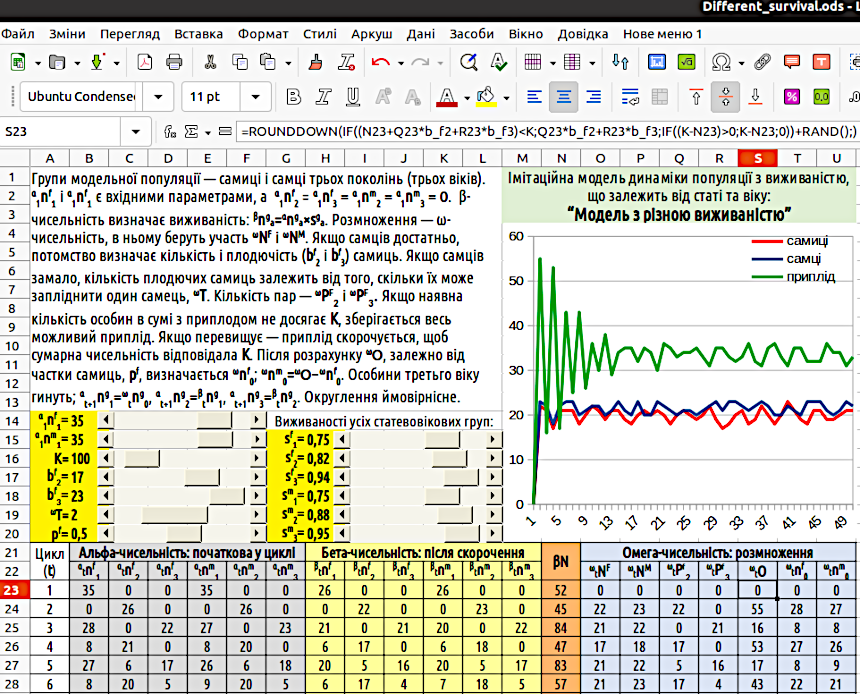
However, this does not mean that such a model does not require improvement. Descriptions of its further modifications follow. Fig. 5.1. General view of the «Model with Variable Survival Rates». Note the formula in cell S23! 5.2. «Reproduction is Hindered by Starvation» At this stage of working with the model described in the previous pages, it is proposed to rebuild it, accounting for the different resource consumption by representatives of different sex-age groups. Surely, a newborn child does not require as many resources as an adult female (woman) or adult male (man)? If individuals in a population differ in the amount of resources they require, we will have to specify the constraints imposed by the environment on population growth differently. We will define this constraint not via the carrying capacity K of the environment, set such that the total population size after reduction βN must not exceed K (i.e., βN ≤ K), but as resource availability V (volume). In this case (in accordance with the rules we have adopted), we will need another notation. We use the letter D (demand) to denote resource demand. Most likely, the resource demand for newborn females and males should be identical: df0 = dm0; in addition to these values, df1, df2, etc. will also have to be specified. Resource demand can be calculated for the model population size at different stages. How to specify resource demands for different individual categories? Select values that seem appropriate to you. Build the model. Observe how the model population behaves depending on the resource demands of different individual categories. It is likely that using the model will help understand how the ratio of initial parameters affects the dynamics of the model population. To begin, let us build a model with reproduction constraints under resource scarcity. We will assume that only as much offspring will be produced as free resources allow. We must emphasize that in this case, population growth is limited not by maximum population size, but by resource scarcity. Therefore, we will name the model we create at this stage of our work «Reproduction is Hindered by Starvation». We will account for the following stages: – alpha population size – initial population size at each cycle; – beta population size – after reduction caused by variable survival; – gamma population size – offspring number in the case of maximum reproduction (γnf0 and γnm0); – omega population size – final population size, which in the case of free resource scarcity may include a smaller number of offspring than the gamma population size (ωnf0 and ωnm0). To calculate the omega population size, the resource demand of all existing individuals before reproduction (βD) and the offspring in the case of maximum possible reproduction (γD) must be calculated. 1. βD ≥ V, i.e., the resource demand of already existing individuals exceeds the amount of resources in the environment; no offspring are produced (ωnf0 = ωnm0 = 0); by the way, in this case, the gamma population size does not even need to be calculated; 2. βD < V, but (βD + γD) > V, i.e., there are sufficient resources for existing individuals, but if all possible offspring are added to the existing individuals, resources will be insufficient; the number of offspring is determined as follows: (ωnf0 + ωnm0) = (V – βD) / df0; 3. (βD + γD) ≤ V, i.e., resources are sufficient for both existing individuals and all their possible offspring; offspring are not limited and equal the gamma population size (ωnf0 = γnf0 and ωnm0 = γnm0).{ "translated_text": "Construct such a model and investigate its dynamics under different values of initial parameters. In what ways is this model better, and in what ways worse, compared to the previous one? 5.3. \"Model with Competitive Reduction\" If you have constructed the model described in the previous step, take another step and build a model with competitive reduction of population size under resource scarcity. To simulate such population reduction, you can apply an algorithm first used in the doctoral dissertation of M. O. Kravchenko. We present this algorithm in a form that incorporates the notation system used in this manual. Unlike previous methods for accounting for constraints on population growth, this algorithm ensures fully realistic model behavior. We consider a population or an HPS (hemiclonal population system) of the green frog hybridogenic complex, as in Kravchenko’s work, or a guild—i.e., a set of different populations using the same resource. The set under consideration includes individuals belonging to different forms, denoted as g (genotypes). In the previous example, there are two forms: females (F) and males (M), but strictly speaking, there can be any number; if their number is k, the different genotypes are g1, g2, g3 ... gk. These genotypes may belong to a single species, like females and males, or to different species, or to the parental species of a hybridogenic complex and their various hybrids. Representatives of each genotype may be grouped into different age classes. If the system under consideration includes max_a age classes, starting from the 0th (newborns), then genotype gg can be represented by the following age classes: gg0, gg1, gg2 ... ggmax_a. A feature of this algorithm is that mortality is divided into two categories: non-competitive mortality and competitive mortality. The metric defining non-competitive mortality is survival (s). Non-competitive mortality does not depend on resource availability and occurs in every cycle under any circumstances; competitive mortality occurs only when the model population is affected by resource scarcity. Logically, non-competitive mortality should be simulated before simulating competitive mortality. For the algorithm under discussion, among other initial parameters, survival values must be set for all groups: sg0, sg1, sg2 ... sgmax_a. This can be done in two different ways: using a table or a function. The first method involves listing each sga value and specifying the corresponding value in the appropriate model cell (for the educational model that students will build, this is the simplest approach). The second approach involves defining a specific function that describes how the survival of each genotype’s representatives changes with age. Specific sga values will then be calculated based on the values of this function. The metric defining competitive mortality is relative competitive ability (c). Values of relative competitive ability for all groups: cg0, cg1, cg2 ... cgmax_a are set in the same way as survival values. Transformations occurring for each group of individuals gga can be described as a transition along a chain of states αnga → βnga → (γnga) → δnga → ωnga. We assume the following: — Alpha-count: population size at the start of the cycle; — Beta-count: population size after non-competitive mortality; — Gamma-count: an auxiliary value, the quota population size in case of reduction, corresponding to competitive ability; — Delta-count: population size after competitive population reduction; — Omega-count: the result of reproduction, i.e., offspring population size. Thus, at the start of each cycle, the population size of each group is αnga. At the start of cycle t, the initial population size αtnga is determined by the population size of the previous age class in the previous cycle. For offspring: αtng1 = ωt−1ng0; if a > 0, αtnga+1 = δt−1nga. At the next stage, non-competitive mortality is simulated, which depends on survival: βtnga = αtnga × sga. At the next step, competitive population reduction is simulated: βtnf1 → δtnf1. Naturally, the most complex part of this model is the competitive mortality algorithm and the calculation of omega-count. To simplify calculations, we can compute intermediate values: the competitive ability-quota population sizes of all groups. We denote these as gamma-counts, and define γtnf1 = βtnga × cga. In addition, two more values must be calculated for further computations: the total resource demand of all individuals before population reduction, βD = Σ(βtnga × dga), and the total resource demand corresponding to the population size of all quota groups, γD = Σ(γtnga × dga) = Σ(βtnga × cga × dga). After calculating these values, we can determine which scenario will govern competitive population reduction. We denote the scenario as W (way, i.e., path or method). W=1, Scenario I: βD ≤ V; resources are sufficient for all, so no competitive population reduction is performed: δnga = βnga. W=2, Scenario II: βD > V and γD ≥ V; resources are insufficient even after quota reduction. In this case, the quota population size should be further reduced proportionally to V/γD: δnga = γnga × V/γD. If, after quota reduction, the total resource demand of the entire set of individuals equals the available resource amount, this formula also applies (since V/γD = 1). W=3, Scenario III: βD > V and γD < V; resources are insufficient for all individuals, but exceed the demand of quota groups. In this case: δnga = βnga − (βnga − γnga) × (βD−V)/(βD−γD). The calculation of omega-count (offspring) can be left as in previous models—for example, the \"Three Generations Model\". You can also use the mechanism applied in the \"Reproduction Inhibited by Starvation\" model, which will result in more effective adjustment of the model population size to the consumption level determined by V. One possible layout of such a model on a LibreOffice Calc sheet, corresponding to the \"Table with Header\" template, is shown in Fig. 5.2. Is it necessary to copy this layout, or must the model be arranged exactly this way? No. However, especially considering previous models, it is clear that the priority here is continuity with what you have done before, and improving the reader’s understanding of the model. You should not copy this option, but create your own, which is clearer and generally better. Fig. 5.2. General view of the model with competitive population reduction under resource scarcity. The formula in cell X27, which describes competitive population reduction, is shown. Naturally, the most complex stage in this model is simulating competitive reduction, and the least intuitively understandable part of this stage is Scenario III. To understand it, the following must be taken into account: (βD−V)/(βD−γD) is the ratio of the resource shortage for the unreduced population size to the difference in resource demand between the unreduced (β) and quota (γ) population sizes. For example, the beta-count (unreduced) requires 500 units of resource, the gamma-count (quota) requires 200 units. Total available resources are 400. The resource shortage for the beta-count is 100 units, the difference in demand between beta- and gamma-counts is 300 units. The ratio (βD−V)/(βD−γD) equals 1/3. This means that one-third of the difference between beta- and gamma-counts must be subtracted from the beta-count: 500 − 300/3 = 400. This population reduction satisfies two conditions: 1) The pre-reduction population size is reduced to a value corresponding to resource availability; 2) The pre-competitive reduction population size of each group βnga is reduced to a post-competitive reduction size δnga such that the proportion of individuals surviving competitive reduction in each group is proportional to the competitive ability of that group’s representatives: δnga/βnga ~ cga. After executing the competitive reduction algorithm, it is useful to calculate the final resource consumption: δU = Σ(δnga × dga). If δU matches V, the reduction has been performed correctly. It must be emphasized that δU will equal V exactly only if calculations are performed without rounding (which is, generally speaking, far removed from biological sense). In the calculations described, you should use either rounding down (for deterministic models, i.e., models where input parameters uniquely determine the result), or rounding after adding a random number (for probabilistic models).
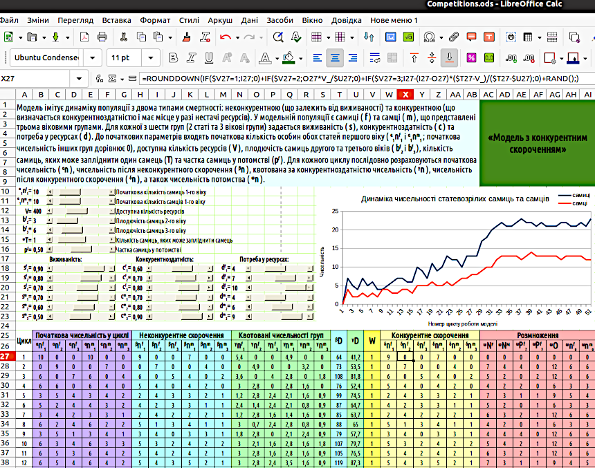
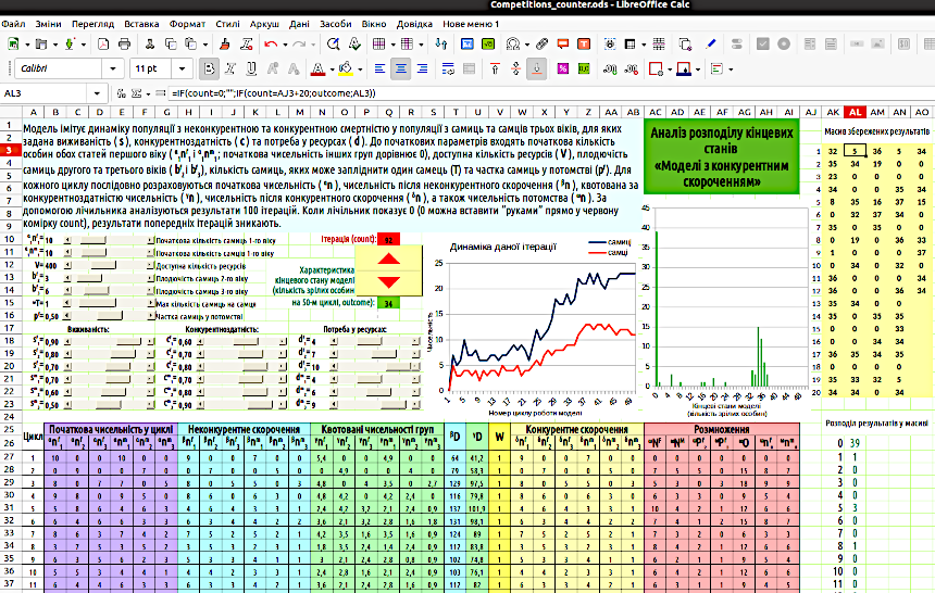
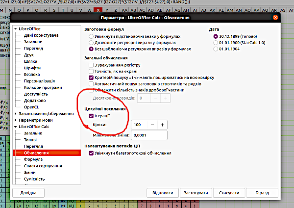
Fig. 5.2 shows a model with probabilistic rounding. 5.4. Analysis of Probability Distributions of Model Final States The renowned French astronomer and mathematician of the late 18th to early 19th century, Pierre-Simon Laplace, believed that the world is determined by its initial state. The \"Laplace's Demon\" is an imaginary entity that knows the coordinates, mass, direction of motion, and speed of all particles in the Universe. According to Laplace’s thought experiment, this entity can calculate past and future states of the Universe for any point in time. For Laplace, the world is deterministic, i.e., its changes are fully determined by its initial state. An important result obtained by modern science is the understanding that the world is not deterministic, but statistical-probabilistic. This is especially evident in quantum mechanics. A unique prediction of a system’s dynamics cannot be derived from its initial state parameters; a future prediction can only take the form of a probability distribution of its future states. The models we build are far simpler than the Universe (which is precisely why their use is meaningful). The first models we built in this course were deterministic. Deterministic models transition to a specific, unambiguous state. People with only a superficial familiarity with models often expect a model to provide an accurate prediction of the dynamics of a natural process. This is most often impossible. The course of natural processes is in fact influenced by a huge number of random events and unpredictable factors. Naturally, a model cannot reflect all the diversity of processes occurring in reality. However, a simulation model can simulate the random course of natural processes to some extent. Such were our models with probabilistic rounding, which we began building starting from Section 3.5. The result of probabilistic modeling will differ each time. By analyzing the distribution of modeling results, we can determine which states the model (given fixed initial parameters) reaches most often, which it reaches rarely, and which it never transitions to. Probabilistic models generate a specific probability distribution of final states. This information is also very valuable for understanding natural processes studied using simulation modeling. You can compare the behavior of deterministic and probabilistic models. For example, take the \"Model with Competitive Reduction\" (provided you built it as shown in Fig. 5.2: with probabilistic rounding). Remove the last element from all formulas of the type =ROUNDDOWN(\"cell_value\"+RAND();): RAND(). The model will become deterministic (and far less interesting...). A probabilistic model is more interesting at least because it yields a somewhat new result each time; it is not predictable in advance. How can you compare deterministic and probabilistic models? Run the probabilistic model for one \"run\", one iteration? This will be insufficient. We will observe different final states. If we recalculate (e.g., using the F9 key), the results of the probabilistic model will change, while those of the deterministic model will remain unchanged. However, the final state of a probabilistic model may be typical or rare. How can this be accounted for? To build a distribution of modeling results, we use an iteration counter (iterations are repetitions, in this case, repeated model runs). To work with the counter, you must enable the iteration mode. This can be done (Fig. 5.3) via the menu Tools / Options / LibreOffice Calc / Calculate. Fig. 5.3. Iteration mode enabled. Enable (if not already enabled) the menu View / Toolbars / Form Controls, the use of which was explained in Section 4.1. Enable \"Design Mode\" and insert the \"Counter\" form control into the model. This control changes the value in the specific cell it controls with each click. Assign the cell controlled by the counter the name counter. We now need cells in which to store the results of each iteration. For each of these cells, we could specify which counter value corresponds to the cell (one cell stores the modeling result when the counter reads 1, another when it reads 2, and so on). However, the simplest approach is to create a row of cells with natural numbers (enter 1 in one cell, 2 in another, and drag the series), then write a formula in the result storage cells with a condition that the counter reading equals the value of the cell in the same row. Fig.
5.4 shows such an option: a row of 20 numbered cells \"services\" 100 result cells. In the first column of result cells, the counter reading is compared to the number cell values; in the second column, 20 is added to the number cell values, in the third 40, and so on. The total number of \"sexually mature\" individuals (\"two-year-olds\" and \"three-year-olds\") is selected to characterize the modeling result. This result is reflected in the cell named outcome. In the result storage array, each group of cells contains formulas similar to the one shown in Fig. 5.4: =IF(count=0;\"\";IF(count=AJ3+20;outcome;AK3)). What does this formula do? It is located in cell AK3 and contains a reference to the cell itself. It is precisely to enable such calculations that iterations must be allowed as shown in Fig. 5.3. This formula works as follows: if the counter cell (count) contains 0, all result recording cells are cleared (the expression \"\" corresponds to an empty cell). If the counter value matches the number cell value (AJ3; since we are analyzing the formula in the second column, AJ3+20), the modeling result from the outcome cell is placed into the result recording cell. If the counter value is anything else, the value of cell AK3 equals itself, i.e., it does not change. By the way, note that the term \"iteration\" is used in two different senses in this section. In Fig. 5.3, it denotes a formula referring back to the cell containing the formula itself. When we refer to the iteration counter, we mean repeated simulations with the same input parameters. How to build a distribution of modeling results? The model in Fig. 5.4 uses the following approach. In column AK, starting from row 26, possible modeling results are listed. Cell AK26 contains the formula =MIN(AK3:AO22), which selects the smallest obtained value; below are formulas that add 1 to this value sequentially. Column AL counts the number of cells in the result storage array that contain the obtained value. The formula =COUNTIF(range;value) is used for this. Range is the array, value is the value of the left cell. For example, cell AL26 contains the formula =IF(count=0;\"\";COUNTIF(AK$3:AO$22;AK26)). The resulting distribution is displayed as a histogram. Can you explain why the distribution has such a strange appearance? More than a third of iterations ended with zero population size. There is a specific group of iterations whose results are distributed around the value 34. There are also scattered results located between zero and the described group of \"successful\" iterations. Why is this? Fig. 5.4.