
Creation of Worlds — 02. Example of a simple model: simulation of exponential growth
We will begin mastering modeling in LO Calc with a simulation model describing exponential population growth. Completing this task will allow one to understand how formulas are entered and «stretched» in LO Calc, to grasp the difference between relative and absolute addressing, and to examine the basic foundations...
2. Example of a Simple Model: Simulation of Exponential Growth
2.1. Mastering Calc: Using Cell Addresses, Entering Formulas
As everyone who has studied ecology knows, the simplest model describing population growth is the exponential model (Fig. 2.1).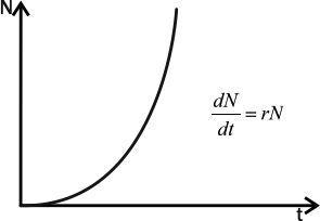
Fig. 2.1. Dynamics of exponential growth (Shabanov, Kravchenko, 2009)
In the model shown in the figure, N is the population size, t is time, r is the reproductive potential (Malthusian parameter), and dN/dt is the change (increase) in population size. In general, this model reflects the simplest fact: the possible increase in population size is proportional to its size. The study of exponential growth was begun by Leonardo Fibonacci (1170–~1250) and Thomas Malthus (1766–1834). The figure presents an analytical model. In it, growth is described using a single-valued function.
Let us create a simulation model in LibreOffice Calc that describes exponential growth. Further examples are given for working with the Ukrainian-language version of LibreOffice Calc 6 for Linux; using other versions of LO Calc may have its own peculiarities.
A LO Calc sheet is a table consisting of columns and rows. In the most common addressing mode (so-called A1), columns are denoted by Latin letters (or their combinations), and rows by numbers. There is also another addressing style (so-called R1C1); to switch between these styles, go through "Tools / Options / LibreOffice Calc / Formula" (here and below, sequences of selected options in the LO Calc menu are shown in italics).
In this handout, work with LO Calc tables is described either using examples of simple tables inserted into the text (such tables will be used only in the initial part of the handout; it can be hoped that as the reader's skills improve, they will become redundant), or illustrated by screenshots (captured window images). First of all, it is necessary to understand the basic principles of relative and absolute addressing in LO Calc.
Let us create a LO Calc file. First of all, let us set up the cells into which we will enter the basic parameters (Table 2.1).
Table 2.1. Beginning of constructing a model describing exponential growth
| A | B | C | D | |
| 1 | 0N= | 1000 | ||
| 2 | r= | 0,2 | ||
| 3 | ||||
| 4 | 0 | 1000 {=B1} | ||
| 5 | 1 | |||
| 6 | 2 | |||
| 7 | 3 |
Cells A1 and A2 (we will denote cell addresses, rows, and columns in bold), in which the designations of the initial values are given, are not used in calculations. They are needed not for the operation of the model itself, but for the user, so that they understand where what is. 0N is the designation of the initial size. To convert 0 to a subscript, let us use the LO Calc sidebar. The sidebar may be collapsed; in that case, it should be expanded by selecting the "Properties" tab (Fig. 2.2). If the sidebar is not even present in its collapsed form, it should be called: "View / Sidebar". To change font parameters, it is necessary to select the symbol to which specific formatting should be applied, and specify this formatting in the sidebar (Fig. 2.3).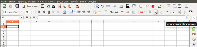
Fig. 2.2. The LO Calc sidebar located on the right is collapsed; it needs to be expanded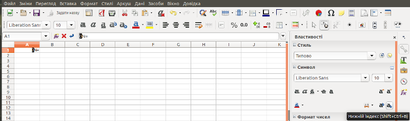
Fig. 2.3. A symbol is selected in cell A1; its properties can be changed using the LO Calc sidebar
The same result can be achieved by selecting the required symbols in the cell or in the formula bar and going through "Format / Text / Subscript". You can also use the keyboard shortcut indicated on the hint (the label that appears when a certain object is selected) in Fig. 2.3.
In the corresponding cells of column B, let us enter the values of the initial parameters specified in Table 2.1.
In column A (indenting a certain place), let us enter the time scale. For this, it is sufficient to enter the numbers 0 and 1, select them with the cursor, place the cursor in the lower right corner of the formed block, press the mouse button and "drag". LO Calc will fill the necessary area with the continuation of the given arithmetic progression. Sometimes LO Calc's desire to construct arithmetic progressions becomes inconvenient. If you similarly "stretch" a cell into which a certain digit is entered, the program will not repeat the same digit over the entire block, but will construct a progression. To fill the block with the same digit, it will have to be copied to the clipboard, select the block, and execute the "Paste" command. If you "stretch" a cell into which a formula is entered, this formula may remain unchanged, or it may change systematically — depending on how it is specified (see below).
In column B, we will place the simulation of exponential growth. In the cell corresponding to the beginning of the simulation, let us enter the formula =B1. If the content of a cell begins with the sign =, LO Calc treats it as a formula. In this handout, formulas will be shown in curly braces on a yellow background, after the value that LO Calc shows in that cell. Thus, the entry "1000{=B1}" means that LO Calc shows the value 1000 in this cell, and this is set by the formula =B1.
One way to enter a formula into cell B4 is this: enter into it (selecting it with the cursor) the sign =, then go to the formula bar (clicking on it), and, placing the cursor after the sign =, select the target cell (B1). After this, it is important not to click the cursor on various places in the table (so that LO Calc does not arbitrarily edit the formula), but to exit the editing mode by pressing Enter.
When this cell is selected, its value is shown in the cell itself, and the formula entered into the cell is shown in the formula bar (Fig. 2.4). If you move the cursor to the formula bar, the cells referenced by the formula will be "highlighted" (Fig. 2.5).
By the way, by default LO Calc aligns text content of cells to the left edge of the cell, and numeric content to the right edge. In the model shown in Fig. 2.4, the alignment in cells A1—B2 was changed to better show the connection between the designation of the initial parameter and its value. In addition, these cells are in bold.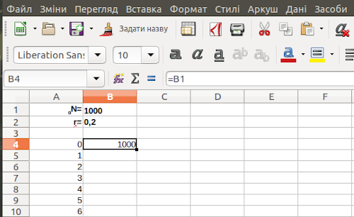
Fig. 2.4. Cell B4 is selected with the cursor; the cell shows its value, and the formula bar shows the formula entered into this cell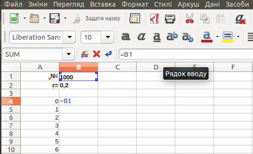
Fig. 2.5. The cursor is in the formula bar; the cell referenced by this formula is highlighted. You should exit this mode by pressing Enter or Esc! Clicking on other cells in formula editing mode will lead to corrupting the formula
Now let us determine what the population size will be after a single time interval. For this, let us enter into cell B5 a formula corresponding to the expression N1=0N+r*0N (Table 2.2).
Table 2.2. Filling the cells of the model
| A | B | C | D | |
| 1 | 0N= | 1000 | ||
| 2 | r= | 0,2 | ||
| 3 | ||||
| 4 | 0 | 1000 {=B1} | ||
| 5 | 1 | 1200 {=B4+B4*B2} | ||
| 6 | 2 | |||
| 7 | 3 |
In cell B6, according to this logic, the formula {=B5+B5*B2} should be located. This and subsequent formulas can be entered into cell B6 and all subsequent ones manually, but this is too complicated. Obviously, all subsequent expressions in column B are analogous to what is entered in cell B5. Can we "stretch" it over the entire column?
Select cell B5 in Calc and stretch it to cell B6. In cell B6, the formula {=B5+B5*B3} will appear. When "stretching", LO Calc shifted all addresses mentioned in the formula. As for the reference to the previous cell in the row (B5 for cell B6) this is absolutely correct, but for the reference to the parameter value r (B3 for cell B2) — it is incorrect.
The thing is that for references in the formula, we used relative addressing. Actually, when cell B5 contains the formula {=B4+B4*B2}, it means {=the_cell_above+ the_cell_above*three_cells_above}. To indicate that a specific cell is needed, the reference to which should be the same regardless of which place in the sheet the formula is located, absolute addressing should be used. In the addressing system we are considering in this example, it is denoted by the dollar sign: {=B4+B4*$B$2}. By the way, in our case (when "stretching" the formula occurs within a certain column) the record given is analogous to the variant {=B4+B4*B$2}. However, in the second of these cases, if you "stretch" such formula into another column, the reference will point to the second row of this new column. Obviously, the reference to the previous cell in the population size calculation row should remain relative.
In some cases, for selecting relative and absolute addressing in LO Calc, the command "Sheet / Change Reference Type" or its equivalent, the F4 key, may be useful. Press this key and look at how the formula changes: there is a cyclic transition between four states:
— relative addressing both in columns and in rows;
— absolute addressing both in columns and in rows;
— relative addressing in columns and absolute in rows;
— absolute addressing in columns and relative in rows.
Such switching is often convenient. However, for the case we are considering, switching via F4 is inconvenient, because in one formula it is necessary to combine a relative reference (for the previous value in the row) and an absolute reference (for one of the initial parameters).
By the way, when using the R1C1 reference style, the same formula will look like this: {=R[-1]C+R[-1]C*R2C}; relative references are in square brackets, absolute ones are not. R[-1]C in this case means a reference to the cell one row above in the same column where the formula is located, and R2C is a reference to the cell in the second row of the same column where the formula is located.
However, in our example, we use traditional references. In that case, by "stretching" the formula from cell B5 over the entire column (probably longer than shown in the example in Table 2.3), we will get the necessary row of values.
Table 2.3. Result of "stretching" the formula with absolute addressing in rows
| A | B | C | D | |
| 1 | 0N= | 1000 | ||
| 2 | r= | 0,2 | ||
| 3 | ||||
| 4 | 0 | 1000 {=B1} | ||
| 5 | 1 | 1200 {=B4+B4*B$2} | ||
| 6 | 2 | 1440 {=B5+B5*B$2} | ||
| 7 | 3 | 1728 {=B6+B6*B$2} |
Thus, the dependence of the model population size on time, corresponding to exponential growth, is constructed.
2.2. Graphical Representation of the Obtained Dependence
We have obtained a series of numbers describing the dynamics of population size growing according to the exponential model. This dynamics will be much easier to interpret if it is represented on a graph. Probably, to make the graph clearer, the columns should be given titles. Let us enter the symbol t in cell A3, and N in B3. Let us center these designations, make them bold. Let us select with the mouse the range starting from these titles and covering two columns with calculations to the very end. Let us select the command "Insert / Chart..." (or select the corresponding button-icon on the toolbar). Let us select the type of chart shown in Fig. 2.6.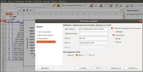
Fig. 2.6. Selecting the type of chart that will be inserted into the LO Calc sheet
By pressing the "Next >>" button, we will be able to set some properties of the created graph. To have its axes labeled, it is worth using both the first row and the first column as labels (Fig. 2.7).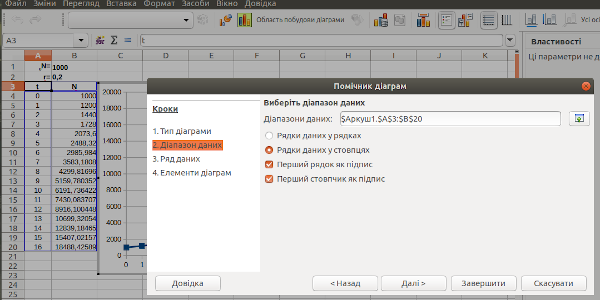
Fig. 2.7. Editing the graph parameters
In one of these dialogs, you can enter the overall title of the graph (Fig. 2.8). Figure out independently the effects of applying other elements of the dialog.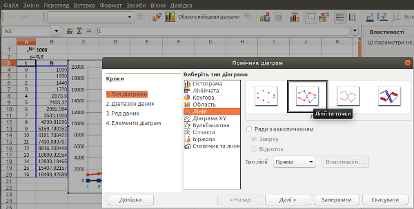
Fig. 2.8. Editing labels on the created graph
The obtained result can be seen in Fig. 2.9 (the unnecessary designation of the value reflected on the graph has been removed). Among other things, the model should be given a meaningful name (it can also be seen in Fig. 2.9).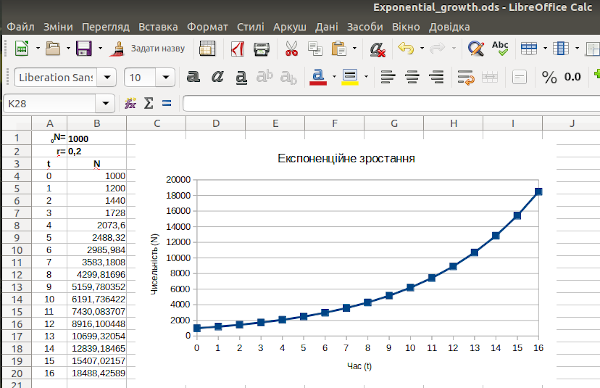
Fig. 2.9. Almost ready... However, the created model still needs some improvement
2.3. Improving the Graph
In LO Calc, two different variants of chart selection should be distinguished. In Fig. 2.10, the chart itself is selected with a simple mouse click; it is marked with green markers at the corners and in the middle of the sides. In Fig. 2.11, elements of the chart can be selected; for this, you should enter chart editing by double-clicking; note that the markers have become dark blue.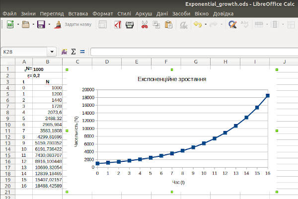
Fig. 2.10. The chart is selected; in this state, it can be scaled, moved, etc.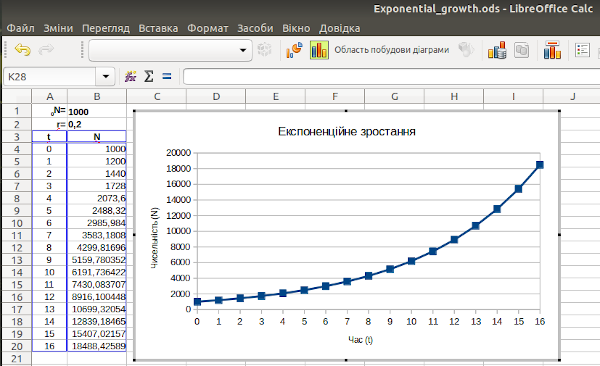
Fig. 2.11. Editing the chart; in this state, its elements can be changed
In chart editing mode, you can right-click on the axis and select the "Format Axis..." option; you can also right-click and immediately get to the dialog shown in Fig. 2.12. There you can change the range reflected on the axis (by unchecking "Automatic"). Try to rebuild the scale in logarithmic mode by placing the corresponding checkmark, as shown in Fig. 2.12. How will the appearance of the graph change? How to explain this?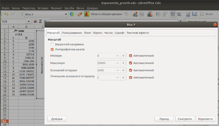
Fig. 2.12. Editing the properties of the graph axis
The last step remains. To be able to use the model, it is necessary to add necessary explanations to it. Let us select all cells occupied by the model. Let us take the cursor by the side edge of the block and drag it (Fig. 2.13). Let us free a couple of rows for the label. This can also be done differently: select the headers of two rows, right-click on them and choose to insert rows (Fig. 2.14). The result of the changes shown in Fig. 2.14 is identical.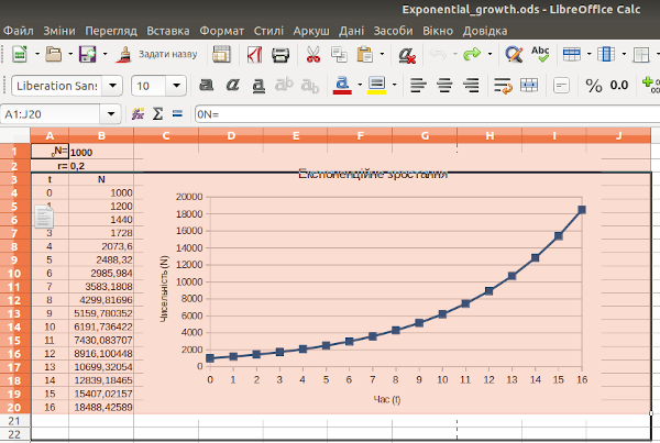
Fig. 2.13. Moving the block of cells; the cursor "drags" the selected block, which also includes the chart, by the left side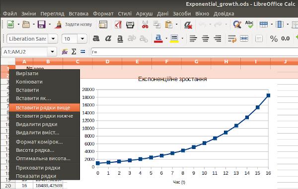
Fig. 2.14. To get free space, you can simply add the necessary rows
It is necessary to note a certain "bug" (in computer slang — an error, from Engl. bug) in LO Calc. When moving the graph, it will most likely "slip" — lose correspondence to those data ranges that should be reflected on it (an example is shown in Fig. 2.15). If this does not happen to you — then good; but this error makes it possible to get acquainted with an important graph editing dialog.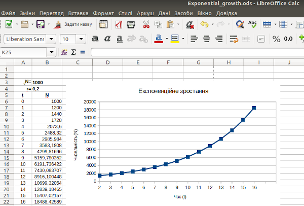
Fig. 2.15. The data range specified for the graph does not correspond to its new location; this range needs to be changed
Let us enter graph editing mode (select it as in Fig. 2.11), and after right-clicking, select the "Data Ranges..." option (Fig. 2.15).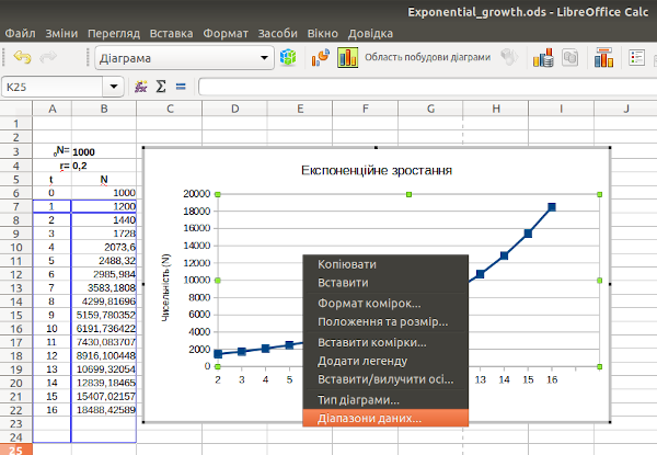
Fig. 2.16. The menu shown in the figure gives wide possibilities for graph editing. Figure out which elements of it are responsible for what!
What should the range reflected on the graph be? We have already labeled the axes, and the option "First row as label" (Fig. 2.17) has lost its meaning. Let us remove the checkmark in this option, and set the range from row 6 to row 22.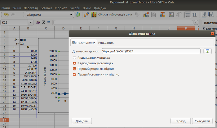
Fig. 2.17. Everything is clear! Data ranges do not correspond to the location of the calculations
Here is what should come out (Fig. 2.18).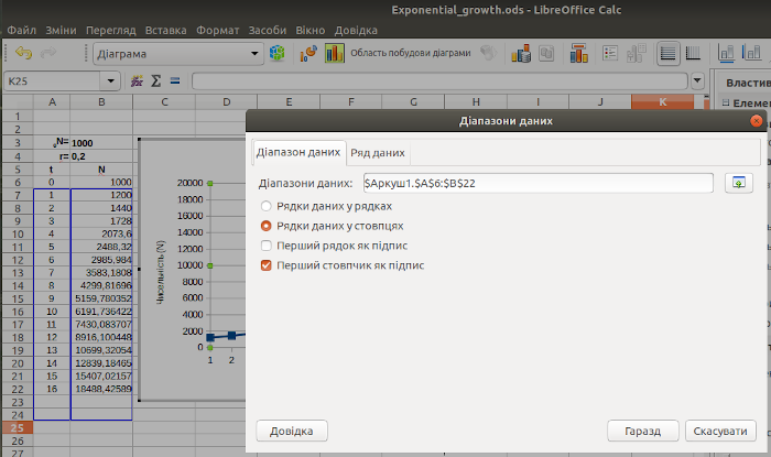
Fig. 2.18. The ranges are corrected, the checkmark on the "First row as label" option is removed
Now we can beautify our model. Let us use for this a normal, not logarithmic scale.
Let us select the cells of the two top rows, in which we will place the explanations. Let us merge them into one ("Format / Merge Cells / Merge and Center Cells"). Let us enter into the merged cell a title that explains what exactly and how is modeled on this sheet. If the text does not fit in one line, you should right-click on the merged cell to call the context menu, in which select the "Format Cells" option. In the "Alignment" tab, you should put a checkmark in the "Wrap text" checkbox. The text in the cell will take on a neat appearance. Let us add a couple more cosmetic changes, reflected in Fig. 2.19. Let us put the initial parameters in a frame; let us apply color fill (figure out yourself how to do it!), change the color and markers on the graph (in chart element editing mode, right-click on the graph, "Data Series... / Line", where you can select the color and marker icons), etc.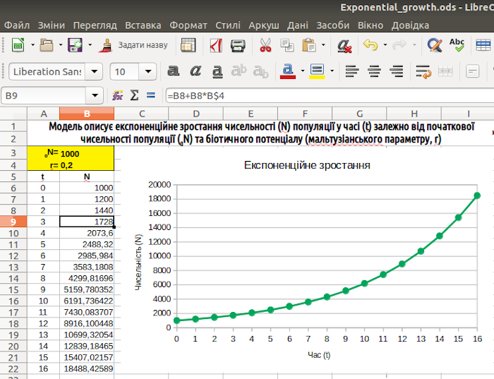
Fig. 2.19. The simulation model is ready!
2.4. Intermediate Summaries
Note: in the model shown in Fig. 2.19, we can see the following structural elements:
— information field;
— input parameters;
— transformation system (step-by-step calculations of population size that simulate the sequence of stages of its growth);
— visualization of output parameters (graph).
Such a model can already be used, for example, when studying the patterns of exponential growth. Even more important is the fact that this model can be extended by adding additional assumptions and conditions that will complicate it and bring it closer to reality.
When bringing the model to "finished" form, the following capabilities of LO Calc were used:
— subscript in the designation 0N;
— "stretching" of arithmetic progression;
— work with the simplest formulas;
— "stretching" of formula;
— use of absolute and relative addressing;
— construction and editing of graph;
— dragging of blocks;
— adding of rows;
— merging of cells;
— setting up text wrapping;
— formatting of cell borders, as well as color fill of cells.
The obtained model can be downloaded from the site, but it is better to create it yourself.
| A | B | C | D | |
| 1 | 0N= | 1000 | ||
| 2 | r= | 0,2 | ||
| 3 | ||||
| 4 | 0 | 1000 {=B1} | ||
| 5 | 1 | |||
| 6 | 2 | |||
| 7 | 3 |
Cells A1 and A2 (we will denote cell, row, and column addresses in bold font), which contain the initial values, are not used in calculations. They are needed not for the model's operation itself, but for the user to understand where everything is located. 0 N is the notation for the initial population size. To convert 0 to a subscript, we will use the LO Calc sidebar. The sidebar can be collapsed; if so, it needs to be expanded by selecting the "Properties" tab (Fig. 2.2). If the sidebar is not even in a collapsed form, it needs to be called up: "View / Sidebar". To change font parameters, select the character to which the specific formatting should be applied and specify this formatting in the sidebar (Fig. 2.3). Fig. 2.2. The LO Calc sidebar, located on the right, is collapsed; it needs to be expanded. Fig. 2.3. In cell A1, a character is selected; its properties can be changed using the LO Calc sidebar. The same result can be achieved by selecting the desired characters in the cell or in the formula bar and following the path "Format / Text / Subscript". You can also use the keyboard shortcut indicated in the tooltip (labels that appear when an object is selected) in Fig. 2.3. In the corresponding cells of column B, enter the values of the initial parameters indicated in Table 2.1. In column A (leaving some space), enter the time scale. To do this, it is sufficient to enter the numbers 0 and 1, select them with the cursor, place the cursor in the bottom right corner of the resulting block, press the mouse button, and "drag". LO Calc will fill the required area with the continuation of the specified arithmetic progression. Sometimes LO Calc's desire to create arithmetic progressions becomes inconvenient. If you "drag" a single cell containing a specific number in the same way, the program will not repeat the same number for the entire block but will create a progression. To fill the block with the same number, you will have to copy it to the clipboard, select the block, and execute the "Paste" command. If you "drag" a cell containing a formula, this formula may remain unchanged, or it may change predictably, depending on how it is defined (see below). In column B, we will simulate exponential growth. In the cell corresponding to the start of the simulation, enter the formula =B1. If the content of a cell starts with an = sign, LO Calc treats it as a formula. In this outline, formulas will be shown in curly braces on a yellow background, after the value that LO Calc displays in that cell. Thus, the entry "1000 {=B1}" means that LO Calc displays the value 1000 in this cell, and this is defined by the formula =B1. One way to enter a formula into cell B4 is as follows: enter the = sign into it (with the cursor selected), then go to the formula bar (by clicking on it), and, placing the cursor after the = sign, select the target cell (B1). After this, it is important not to click the cursor in different places in the table (so that LO Calc does not edit the formula arbitrarily) but to exit editing mode by pressing Enter. When this cell is selected, its value is displayed in the cell itself, and the entered formula is displayed in the formula bar (Fig. 2.4). If you move the cursor to the formula bar, the cells referenced by the formula will be "highlighted" (Fig. 2.5). By the way, by default, LO Calc aligns text content of cells to the left border of the cell, and numerical content to the right border. In the model shown in Fig. 2.4, the alignment in cells A1-B2 has been changed to better show the relationship between the initial parameter notation and its value. In addition, these cells are highlighted in bold. Fig. 2.4. Cell B4 is selected by the cursor; its value is displayed in the cell, and the formula entered into this cell is displayed in the formula bar. Fig. 2.5. The cursor is in the formula bar; the cell referenced by this formula is highlighted. Exit this mode by pressing Enter or Esc! Clicking on other cells while editing a formula will clutter the formula. Now let's determine the population size after a unit time interval. To do this, enter the formula corresponding to the expression N 1 = 0 N+r* 0 N (Table 2.2) into cell B5. Table 2.2. Filling in the model cells.
| A | B | C | D | |
| 1 | 0N= | 1000 | ||
| 2 | r= | 0,2 | ||
| 3 | ||||
| 4 | 0 | 1000 {=B1} | ||
| 5 | 1 | 1200 {=B4+B4*B2} | ||
| 6 | 2 | |||
| 7 | 3 |
In cell B6, according to this logic, the formula {=B5+B5*B2} should be located. This and subsequent formulas can be entered into cells B6 and all subsequent ones manually, but this is too complicated. It is obvious that all subsequent expressions in column B are analogous to what is entered in cell B5. Can it be "stretched" to the entire column? Select cell B5 in Calc and stretch it to cell B6. In cell B6, the formula {=B5+B5*B3} will appear. When "stretching", LO Calc shifted all the addresses mentioned in the formula. Regarding the reference to the previous cell in the series (B5 for cell B6), this is absolutely correct, and for the reference to the value of parameter r (B3 for cell B2), it is incorrect. The fact is that we used relative addressing for the references in the formula. In fact, when cell B5 contains the formula {=B4+B4*B2}, it means {=cell_above+cell_above*cell_three_above}. To indicate that a specific cell is needed, the reference to which should be the same regardless of where the formula is located on the sheet, absolute addressing should be used. In the addressing system we are considering in this example, it is denoted by a dollar sign: {=B4+B4*$B$2}. By the way, in our case (when "stretching" the formula within a specific column), the given entry is also analogous to {= B4+B4*B$2}. However, in the second of these cases, if such a formula is "stretched" to another column, the reference will point to the second row of this new column. It is obvious that the reference to the previous cell in the population size calculation series should remain relative. In some cases, to select relative and absolute addressing in LO Calc, the command "Sheet / Change Link Type" or its equivalent, the F4 key, may be useful. Press this key and observe how the formula changes: there is a cyclic transition between four states: - relative addressing for both columns and rows; - absolute addressing for both columns and rows; - relative addressing for columns and absolute for rows; - absolute addressing for columns and relative for rows. Such switches are often convenient. However, for the case we are considering, switching using the F4 function is inconvenient because in one formula, a relative reference (for the previous value in the series) and an absolute reference (for one of the initial parameters) should be combined. By the way, when using the R1C1 reference style, the same formula will look like this: {=R[-1]C+R[-1]C*R2C}; relative references are in square brackets, absolute ones are not. R[-1]C in this case means a reference to the cell one row above in the same column where the formula is located, and R2C is a reference to the cell in the second row of the same column where the formula is located. However, in our example, we are using traditional references. In this case, by "stretching" the formula from cell B5 to the entire column (likely longer than in the example shown in Table 2.3), we will get the required series of values. Table 2.3. Result of "stretching" the formula with absolute row addressing.
| A | B | C | D | |
| 1 | 0N= | 1000 | ||
| 2 | r= | 0,2 | ||
| 3 | ||||
| 4 | 0 | 1000 {=B1} | ||
| 5 | 1 | 1200 {=B4+B4*B$2} | ||
| 6 | 2 | 1440 {=B5+B5*B$2} | ||
| 7 | 3 | 1728 {=B6+B6*B$2} |
Thus, the dependence of the model population size on time, corresponding to exponential growth, has been constructed. 2.2. Graphical representation of the obtained dependence We have obtained a series of numbers describing the population dynamics of a growing population according to the exponential model. This dynamics will be much easier to interpret if it is displayed on a graph. Probably, to make the graph clearer, the columns should be given headers. Enter the symbol t into cell A3, and N into B3. Center these labels and make them bold. Select the range with the mouse, starting from these headers and covering two columns with calculations up to the very end. Choose the command "Insert / Chart..." (or select the corresponding icon button on the toolbar). Select the chart type shown in Fig. 2.6. Fig. 2.6. Selecting the chart type to be inserted into the LO Calc sheet. By clicking the "Next >>" button, we can set some properties of the chart being created. To have its axes labeled, it is advisable to use both the first row and the first column as labels (Fig. 2.7). Fig. 2.7. Editing chart parameters In one of these dialogs, you can enter a title for the entire chart (Fig. 2.8). Figure out the effects of applying other dialog elements yourself. Fig. 2.8. Editing labels on the chart being created. The result obtained can be seen in Fig. 2.9 (the redundant notation of the value displayed on the chart has been removed). Among other things, the model should be given a meaningful name (it can also be seen in Fig. 2.9). Fig. 2.9. Almost ready... However, the created model still needs some improvement. 2.3. Chart enhancement In LO Calc, two different ways of selecting a chart should be distinguished. In Fig. 2.10, the chart itself is selected with a simple mouse click; it is marked with green markers at the corners and in the middle of the sides. In Fig. 2.11, chart elements can be selected; to do this, double-click to enter chart editing mode; note that the markers have turned dark blue. Fig. 2.10. The chart is selected; in this state, it can be scaled, moved, etc. Fig. 2.11. Editing the chart; in this state, its elements can be changed. In chart editing mode, you can right-click on an axis and select the "Format Axis..." option; you can also right-click and immediately access the dialog shown in Fig. 2.12. There you can change the range displayed on the axis (by unchecking "Automatic"). Try rebuilding the scale in logarithmic scale by setting the corresponding checkbox, as shown in Fig. 2.12. How will the chart look? How to explain this? Fig. 2.12. Editing chart axis properties The last step remains. To make the model usable, it needs to be supplemented with the necessary explanations. Select all cells occupied by the model. Grab the side edge of the block with the cursor and drag it (Fig. 2.13). Leave a couple of rows for the caption. The same can be done differently: select the headers of two rows, right-click on them and choose to insert rows (Fig. 2.14). The result of the changes shown in Figs. 2.13 and 2.14 is identical. Fig. 2.13. Moving a block of cells; the cursor "drags" the selected block, which also includes the chart, by its left side. Fig. 2.14. To get free space, you can simply add the necessary rows. It should be noted that there is a "bug" (in computer jargon, an error, from the English word bug - insect) in LO Calc. When moving a chart, it is very likely to "slide" - lose correspondence with the data ranges that should be displayed on it (example shown in Fig. 2.15). If this does not happen to you, then good; but this error provides an opportunity to get acquainted with an important chart editing dialog. Fig. 2.15. The data range specified for the chart does not correspond to its new location; this range needs to be changed. Enter chart editing mode (select it as in Fig. 2.11), and after right-clicking, select the "Data Ranges..." option (Fig. 2.15). Fig. 2.16. The menu shown in the figure provides wide possibilities for editing the chart. Figure out what its elements are responsible for! What should be the range displayed on the chart? We have already labeled the axes, and the "First row as label" option (Fig. 2.17) has lost its meaning. Uncheck this option and set the range from the 6th row to the 22nd. Fig. 2.17. Everything is clear! The data ranges do not correspond to the location of the calculations. This is what it should look like (Fig. 2.18). Fig. 2.18. Ranges corrected, "checkbox" for "First row as label" unchecked. Now we can beautify our model. Let's use a regular, not logarithmic, scale. Select the cells of the two top rows where we will place the explanations. Merge them into one whole ("Format / Merge Cells / Merge and Center Cells"). Enter a title in the merged cell that explains what and how is being modeled on this sheet. If the text does not fit on one line, right-click on the merged cell to bring up the context menu, where select the "Format Cells" option. On the "Alignment" tab, check the "Wrap text" box. The text in the cell will look neat. Let's add a couple more cosmetic changes shown in Fig. 2.19. Let's put the initial parameters in a frame; give them a color fill (figure out how to do this yourself!), change the color and markers on the chart (in chart element editing mode, right-click on the chart, "Format Data Series... / Line", where you can choose the color and marker icons), etc. Fig. 2.19. The simulation model is ready! 2.4. Intermediate conclusions Note: in the model shown in Fig. 2.19, we can see the following structural elements: - information field; - input parameters; - transformation system (step-by-step calculations of population size simulating the sequence of its growth stages); - visualization of output parameters (chart). Such a model can already be used, for example, when studying the patterns of exponential growth. Even more important is that this model can be expanded by adding additional assumptions and conditions that will complicate it and bring it closer to reality. When bringing the model to a "marketable" appearance, the following LO Calc capabilities were used: - subscript in the notation 0 N; - "stretching" of arithmetic progression; - working with the simplest formulas; - "stretching" formulas; - using absolute and relative addressing; - building and editing charts; - dragging blocks; - adding rows; - merging cells; - setting up text wrapping; - formatting cell borders, as well as filling cells with color. The obtained model can be downloaded from the website, but it is better to create it yourself.