Lecture
Creation of Worlds — 01. Introduction to the Simulation Modelling Course
The first chapter of the textbook «Creation of Worlds»: simulation modelling of supra-organismal systems in spreadsheets and R.
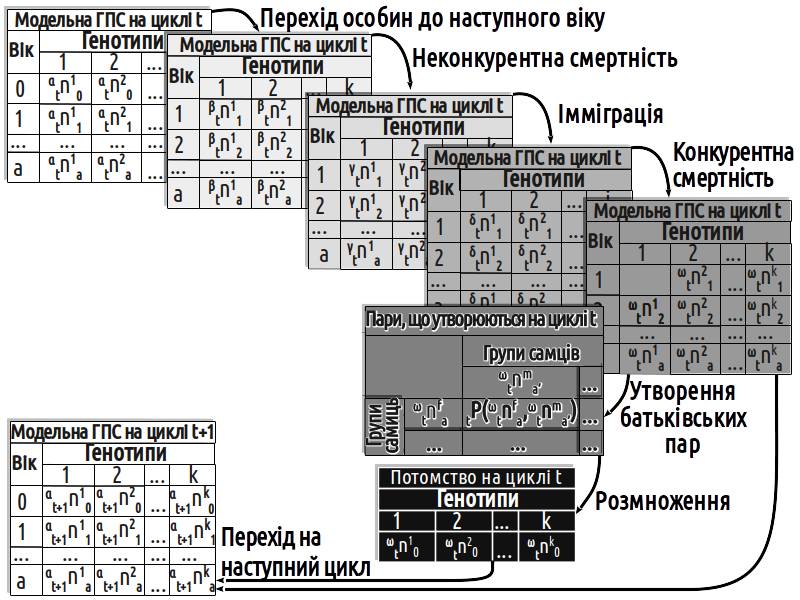
1. Introduction to the Simulation Modelling Course 1.1. Purpose and Features of the Course I heard — I forgot. I saw — I remembered. I did — I understood. (Attributed to Confucius) This course can be called by various names. Probably the most precise title would simply be "Simulation Modelling of Supra-Organismal Systems Using LO Calc or R", but the author finds it most pleasing to think of this course as a course in the creation of worlds. The supra-organismal system models we create are, after all, separate virtual worlds in which model populations will live, are they not? This course has been taught to students of the Department of Zoology and Animal Ecology (first-year Master's students) at Kharkiv V. N. Karazin National University since 2013; since 2021, its expanded form (using the R environment) is to be studied by those doctoral students for whom it will be necessary for carrying out their dissertation research. At various times this course has been treated either as a special elective or as a section of a large practical course. Here (on this and subsequent pages) resides its online textbook, which is being created and revised "on the fly". The course is designed to develop in students of the Department of Zoology and Animal Ecology the ability to construct simulation models of populations and other supra-organismal (and not only supra-organismal) biosystems (and not only biosystems). The author hopes that the materials presented here may be useful in mastering modelling for other "consumers" as well — from schoolchildren to specialists in other fields. Practice has shown that not only a Master's student can complete this course (at least through chapters 6–7) and begin creating their own models; even some motivated schoolchildren can manage it. Against the backdrop of the successes of such motivated schoolchildren, the chaotic efforts of those Master's students who try to avoid taking this course in the order of its development and increasing complexity — grabbing at fragments that are difficult to understand in isolation from everything else, and encountering failure — appear particularly regrettable. Why is it necessary to build simulation models? First and foremost, in order to understand how the objects of modelling function. Some objects we can "make" (in the sense understood in the epigraph to this section) — for example, we can create an experimental population. But its creation and experimentation with it will be drawn out over a considerable period of time. Some objects cannot be "made" — for example, one cannot create a second biosphere. Yet for both types of objects we can construct simulation models that will contribute to the expansion of our understanding. "After creating a model — and sometimes in the process of its development — we begin to investigate the structure and understand the behaviour of the system, to test how it behaves under certain conditions, to compare different scenarios, and to optimise it. When the optimal solution is found, we can apply it in the real world. In essence, modelling is the search for a solution to a problem in the risk-protected world of models, in which we can make errors, undo operations, return to the past, and start everything anew." (I. Grigoryev) The simulation modelling course can be divided into three stages (which have no sharp boundaries, but differ in the principal character of the activities of students and instructor). Stage I — execution of step-by-step instructions. Students become acquainted with the principal tools used for modelling in the LO Calc environment. They will likely experience surprise: a very short list of commands and tools makes it possible to construct very different simulation models, which sometimes exhibit unpredictable behaviour. During this stage, students must follow step by step the instructions detailed in this course notes. As the expected growth in students' proficiency proceeds, the level of detail in the instructions decreases. Stage II — analysis (and, where possible, improvement) of others' models. Students become acquainted with examples of various simulation models created by the instructor, by other authors, and by other students who have studied and are studying simulation modelling. At this stage one must understand how a given model works, grasp how it can be optimised or extended, and incorporate into one's own repertoire the tools used in the construction of such a model. Stage III — free flight: creation of one's own models. The number of problems for whose solution simulation modelling can be used is truly unlimited. At this stage the instructor introduces students to certain problems that seem interesting to him. Students may themselves propose problems that interest them. At this stage, interesting tasks should be solved through independent work combined with discussion of problems, tools, and results of modelling. Some of the models obtained during this stage, with the agreement of all interested parties, may be used as instructional models for Stage II of the course. Some models created at this stage were published in academic papers or qualification theses and played a certain role in the scientific development of their authors. Once a conceptual model has been developed (the subsystems of the modelled system have been identified, and the structure and nature of the connections between them have been established), it can be implemented in various software environments. The main objective of the course — gaining experience in the construction of simulation models — can best be served by focusing directly on this task using the most accessible software environment: spreadsheets. Of course, the most widespread program for working with spreadsheets (a spreadsheet processor) is Microsoft Excel, part of the Microsoft Office suite. MS Excel is a proprietary program, meaning that its source code is the property of its manufacturer. It is also a commercial product sold by its manufacturer to users. MS Office has a number of analogues belonging to free and open-source software. These packages also include spreadsheet processors. In order for the actions described in this textbook to be performable on any computer, regardless of the operating system installed on it and regardless of whether the user holds a licence for commercial software, the examples given in this book refer to LibreOffice Calc (LO Calc). LO Calc is distributed under a free licence. It should be emphasised that this is not a weakened analogue of Microsoft Office Excel, but an independent software product that surpasses its analogues in many respects. Both LO Calc (sincerely recommended by the author of this course) and MS Excel and other spreadsheet programs offer excellent capabilities for non-professional simulation modelling. They provide an unlimited field in whose cells any values can be placed, linked by the required dependencies, and displayed in graphical form. The author has begun adding to this textbook materials that will enable the R language to be used for simulation modelling. Invaluable assistance in this has already been provided by Kateryna Rykova, who has transformed from a student of the course into its co-author. Thank you to her! The author sincerely thanks the colleagues who have gone through this course, as well as all students who made efforts to master it, for their participation in the development of the course. A number of fragments of this textbook appeared as expanded answers to questions posed by students; a number of errors and "dark" passages were corrected precisely because students reported that they had "stumbled" over them. Moreover, the author will be grateful for linguistic and stylistic editing of this text. 1.2. Basic Concepts A system is an organised, ordered whole; a set of subsystems with a characteristic structure of connections and a shared goal (objective function, optimisation function). In the typical case, the reason for the orderliness of a system is precisely its objective function. For many biological systems the objective function is the maintenance of stability — the capacity to preserve and reproduce essential characteristics over time despite external influences. For example, an organism is a temporary stage in a process that, through natural selection, preserves and reproduces a characteristic mode of interaction with the environment. Modelling is the process of studying (forecasting, etc.) an original system, during which it is replaced by a more convenient (accessible, simple, comprehensible, safe, faster-responding, etc.) model system. The result of modelling, to one degree or another, is the extension to the original system of conclusions obtained through the study of the model. A model is a representation of a system; a system whose essential (from the perspective of the problem under investigation) properties correspond to those of the original system. A simulation model is a model that transitions from one state to another in accordance with a certain set of rules corresponding to the sequence of transformations of the original system. "The concept of 'model' is used in many spheres of human activity and has numerous meanings. However, in a general sense, a model can be defined as a certain artificial construction that is a simplified representation of a real system. The simpler structure of the model is expressed in the fact that only certain properties of the real system, considered essential for the process or phenomenon under investigation, are taken into account in its construction (imagine, for example, a scale model of a building made by an architect). By changing these properties in the model, we can better understand the structure of the real system and, most importantly, predict with a certain probability its behaviour in various situations." (S. E. Mastytsky, V. K. Shitikov) The properties of systems can be divided into two groups: additive and emergent (for more detail, see the ecology textbook). Additive properties of a system are determined by the sum of the properties of its subsystems. Emergent properties arise as a result of the interaction of subsystems and are absent at the level of those isolated subsystems outside their interaction. Even a qualified observer who knows the set of subsystems in a system and the nature of the connections between them often finds himself in a situation where he cannot predict in advance what emergent properties will characterise the system. It can be said that emergent properties of systems often turn out to be difficult to predict and are even frequently counter-intuitive — that is, not what the researcher intuitively expects. Why does this occur? To some extent, this is a consequence of our characteristic mode of thinking. Our thinking is well suited to tracking chains of causes and effects (see "The Chain of Antelope Tracks") but poorly suited to predicting the outcome of the interaction of many processes running simultaneously and influencing one another. Modelling is founded on a phenomenon whose significance was first recognised in Ludwig von Bertalanffy's general theory of systems: systems that have a similar character of connection among their subsystems also have similar emergent properties. In the course of modelling it is extremely important to keep in mind that a model is not the original. The fact that a model has certain properties does not prove that the original has them. As a rule, models cannot be used to prove the correctness of hypotheses describing the original. Why then use modelling? Fortunately, the proof of certain hypotheses is not the only benefit of using a model. It should be noted that the definitive proof of certain hypotheses about reality is impossible for science in general. However, modelling often makes it possible to discover internal contradictions in the assumptions used in the construction of the model. Eliminating these contradictions requires replacing the incorrect initial premises (perhaps with new incorrect assumptions, or, if one is fortunate, with hypotheses that correspond well to reality). Thus, the truth of a model cannot be proved, but it can be verified that the assumptions embodied in the construction of the model do not contradict reality! Models by their nature can be divided into the following groups: — physical (material); — symbolic (ideal): — figurative — cognitive: — mental; — verbal; — schematic (graphical); — mathematical (numerical): — analytical; — simulation. Moreover, simulation models can be characterised by several further significant attributes: structural — functional; discrete — continuous; deterministic — probabilistic (stochastic); static — dynamic. In the broadest sense, the cognition of anything is itself also a form of modelling. Modelling in general is one of the principal functions of our brain. We not only react to the stream of stimuli arriving from outside, but also continuously construct in our psyche a model of reality, which we use for adaptation to it. Our fitness (the measure of our expected contribution to future generations) is determined by the result of our interaction with an extraordinarily complex reality. In order to increase the efficiency of interaction with reality, highly developed animals construct a model of it in their psyche. If this model turns out to be a good one, it enables us to predict the actual course of events (the same course that affects our fitness). Apart from the stream of information provided by our sense organs, and the processing of that stream through the construction of models on its basis, there exist in principle no other modes of interaction between our psyche and the environment. On this basis, everything we do can be represented as the creation and improvement of models. In humans, complex symbolic systems are used to construct models; among other things, this allows different individuals to use and improve shared models of aspects of reality important to them. Physical formulas and physical laws are examples of models. Science is an example of a large-scale model that is jointly maintained and developed. At a certain stage, extra-somatic (extra-bodily) carriers and modelling environments begin to be used for the development of complex models. From this point of view, the mastery of a course within which shared formalised models are collaboratively created and implemented in computer program environments constitutes a type of activity lying on the principal axis of our evolution. "The simulation of systems is a specific form of the cognitive process. The subject of simulation may be systems that actually exist, are being designed, or do not even have a direct relation to reality. The fundamental principle of systems simulation is the obtaining of judgements about the simulated system through experiments with the model. It is precisely experiments with the model that distinguish simulation from other forms of cognition." (M. Straskraba) In the situation where simulation models are employed, the entire modelling process can be divided into four stages: — formalisation of representations concerning the original system; — construction of the model using one or another means; — experimentation with the model; — interpretation of the results of modelling. 1.3. Comparison of Analytical and Simulation Models Mathematical models can be represented as a transformation of input parameters (let us denote their aggregate as X) into output parameters (Y). In this case, the operation of the system of transformations that the model's algorithm defines (let us denote it as W) can be described as follows: W(X)=Y. In other words, a model is a regularity that transforms input parameters into output parameters. In the most general form, one can say that a model relates the values of certain parameters to certain functions. Thus, we need only identify the parameters important to us and configure the settings that determine them. What is the difference between analytical models and simulation models? In the case of analytical modelling, W is a formula or system of equations; in the case of simulation modelling, W is a step-by-step transformation algorithm of the input parameters whose logic corresponds to the processes in the original system. Analytical modelling is a powerful method for solving relatively simple problems that can be expressed in a generalised form. For example, we study the dynamics of a body subjected to a certain force. Having obtained a series of estimates of its state, we can establish that the mass of the body (m), the force acting upon it (F), and the acceleration caused by that force (a) are related by the dependency F=m×a — this regularity is known as Newton's second law. This is an excellent analytical model. It is easy to imagine conditions under which the dynamics of the body would be described with sufficient accuracy by this equation. "The analytical representation is suitable only for very simple and highly idealised problems and objects, which, as a rule, have little in common with real (complex) reality, but possess a high degree of generalisability. This type of model is usually applied to describe the fundamental properties of objects, since the foundation is simple in its essence. Complex objects are rarely amenable to analytical description." (O. I. Babina) Analytical models are also used in ecology. For example, we may assume that the growth of a population follows an exponential model — that is, is proportional to its size, i.e. dn/dt=r×N (where N is the population size and r is the biotic potential, a measure of the individuals' reproductive capacity). This differential equation can be solved: Nt=N0ert. In this case, however, the situation is somewhat different from that in physics. To obtain observational series that precisely correspond to this model is practically impossible. Too many different factors influence the population dynamics of virtually any real population ... For the action of many of these relationships, it is difficult to find a mathematically simple description. What is to be done? "An alternative to analytical models is provided by simulation models <...>. The fundamental distinction between simulation models and analytical models consists in the fact that instead of an analytical description of the relationships between inputs and outputs of the system under investigation, an algorithm is constructed that reflects the sequence of development of processes within the object under investigation, and then the behaviour of the object is 'played out' on a computer. Simulation models are resorted to when the object of modelling is so complex that to describe its behaviour adequately by means of mathematical equations is impossible or difficult. Simulation modelling makes it possible to decompose a larger model into parts (objects, 'pieces') that can be manipulated separately, creating other, simpler or, conversely, more complex models. Thus, the main advantage of simulation modelling compared with analytical modelling is the possibility of solving more complex problems, since a simulation model can be gradually made more complex without a decline in the model's effectiveness." (O. I. Babina) I. Grigoryev (2017) identifies three principal approaches to the construction of simulation models: system dynamics, discrete-event simulation, and agent-based modelling. System dynamics was created by Jay Forrester in the mid-twentieth century. An excellent introduction to this approach is the book by Donella Meadows, "Thinking in Systems". According to this approach, in analysing the dynamics of systems one should identify the main stocks ("accumulators") whose levels define the state of the system, as well as the flows that change these stocks. In such an analysis one must establish the main feedback loops (positive and negative). System dynamics is used for the modelling of systems at a high level of abstraction. Discrete-event simulation represents the model as a chronological sequence of step-by-step (often recursive, i.e. repeating) transitions of the system from one state to another. Each transition models a certain event in the dynamics of the original system and is realised at a certain moment in model time. The overwhelming majority of models in this course realise precisely this approach. Agent-based modelling involves the description of a set of individual objects (agents), each of which realises its behaviour in accordance with pre-specified rules. Most frequently, agent-based models involve interaction among agents with one another. The behaviour of the system proves to be the result of the activities of the individual agents. In this textbook one example of a typical agent-based model belonging to the category of cellular automata will be considered. For example, if we regard a population as a whole, we may use system dynamics or discrete-event simulation. If we wish to simulate different categories of individuals within a population and the different stages of their life or annual cycle, the most adequate approach will prove to be discrete-event simulation. With further detailisation of discrete-event models (in which we wish to track the fate of each individual organism), agent-based modelling may be employed. The following chapters of this textbook demonstrate the gradual transition from the realisation of an analytical model to progressively more complex simulation models. From relatively simple formulas one can pass to the description of a population as a collection of individuals, for each of whom one takes into account age, sex, probability of reproduction with each potential partner, survival probability and its dynamics, potential fecundity and its dynamics, as well as other characteristics that may influence population dynamics. Although such a model employs numerous formulas (for example, to describe changes over time in the various characteristics of an individual), such a model transforms into a system of step-by-step transformations corresponding (in simplified form) to the processes occurring in the original object — that is, into a simulation model. For example, Fig. 1.1 shows how a model works that describes the transformations of hemiclonal population systems (HPS) of the hybridogenetic complex of green frogs (source). Fig. 1.1. The operational logic of a model describing transformations of hemiclonal population systems of green frogs (Shabanov et al., 2019) In the model whose operational logic is shown in the diagram, all individuals belonging to one group and of the same age are considered identical. The aggregate of these groups passes sequentially through several transformations that simulate processes occurring in real population systems of frogs. Representatives of each group are characterised by their own set of survival and reproduction probabilities. Thus, step by step, the simulation model restructures the description of the population system. Occasionally, the conclusions obtained by means of such a model prove useful... 1.4.
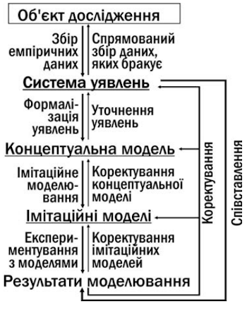
Modelling in Biology At present, modelling has become an entire science (and a practice with elements of creative art), at the intersection of mathematics, computer sciences, and the so-called "subject domains" — sciences that describe research objects, i.e. biology in the case of studying diverse biosystems. The conduct of research at the intersection of disciplines frequently encounters significant difficulties: the characteristic modes of thinking of biologists, mathematicians, and computer specialists differ quite markedly. What seems natural to one specialist simply "does not fit in the head" of another. When modelling is conducted in collaboration with professionals, biologists have to play the role of clients. Practice shows that programmers who create the program itself sometimes find it extremely difficult to adequately reflect what the biologist has in mind. The result is a model that does not work quite as it should, and whose use may lead to erroneous conclusions. A model that does not work quite as it should is, with considerably greater probability, likely to push its user toward errors than a model that does not work at all as it should. There is only one way out: the biologist must himself understand the principles of modelling and be able to construct at least the simplest models. On the one hand, such ability will become one of the prerequisites for successful collaboration with professionals in modelling. Having obtained a non-professional model yourself, you will be able to interact far more effectively with the specialists to whom you commission a model meeting the highest requirements. On the other hand — in a great many cases, modelling skills may enable the biologist to handle many tasks independently, without collaboration with mathematicians or computer specialists. This course is designed to lay the foundation for such a capacity. Most biologists see the benefit of modelling in the possibility of forecasting the dynamics of the original system. However, forecasting does not exhaust the benefit of simulation modelling. Two further mechanisms will be considered here that can make simulation modelling useful for the biologist. The operation of these mechanisms has been verified by the personal experience of the author of this textbook. 1.5. Forecasting The use of models for forecasting is not only the most widespread way of using models, but also the one most easily comprehended by non-specialists. The dynamics of the original system are recorded across a certain set of states (in this context this set can be called the "teacher"). A model is created that produces on the "teacher" the same dynamics as in the original. Such a correspondence of the dynamics of two different systems (the original and the model) can be achieved in various ways. In the case of analytical models, the researcher may hope that he has revealed the essence of the relationship between input and output parameters. In the case of a neural network model, there is typically no hope whatsoever that the model reflects the causal relationships within the original: what matters is that the model is capable of predicting its dynamics. With simulation models the situation lies in a certain sense between these two extremes. In the next stage, the model is used to find out how the original system will behave beyond the set of states that were used for its training. For further discussion it is useful to introduce the concept of phase space as a means of describing the dynamics of the system under investigation. Phase space is defined by those variables that we consider important for describing the state of the system. Such a space can usually be divided into parts corresponding to different types of system states (for example, states of health, illness, dying, and death). Very often the "teacher" represents only part of the phase space of the system, while the predictions the researcher wishes to obtain concern other states. For example, we collect data about the dynamics of the planet's climate system in order to find out whether a catastrophic warming will occur, and if so, when. Present-day climate states we have observed; future warming we have not. Unfortunately, even if the model corresponds well to the dynamics of the original system in the studied part of phase space (on the "teacher"), there are no grounds for confidence that it will be equally adequate for other previously unobserved states. Similar reasons provide grounds for doubt regarding the "nuclear winter" model. Studying the dynamics of the Earth's atmosphere in the observable range of regimes of its functioning, the American and Soviet authors of climate models attempted to determine how this system would behave under conditions that had not been observed. As a result, both groups of authors obtained a scenario of the so-called "nuclear winter". The realism of this scenario has not been sufficiently substantiated (which did not prevent it from playing a notable role in world politics). Thus, although a model forecast cannot be proved, it can be employed in the course of decision-making as one of the possible scenarios. In any case, the "nuclear winter" scenario draws attention to a problem worthy of further investigation. 1.6. Refinement of Conceptions of the Object During Their Formalisation In the typical case, a biologist in his work employs non-formalised ("fuzzy") systems of conceptions about the objects under investigation. Naturally, such systems are also models. The "fuzziness" of such models manifests itself, in particular, in the fact that different aspects of such conceptions may contradict one another. In order to construct a simulation model, the researcher must formalise his conceptions — that is, translate them into a non-contradictory finite set of unambiguous assertions. At this stage one can speak of a formalised conceptual model. Such a model identifies within the original system a number of subsystems and formulates assumptions about the nature of the connections among them. The formalisation of conceptions in the creation of a conceptual model is not a simple task. It is evident that reality is more complex and richer than any schema, and in the course of formalising the initial conceptions, the reflection of reality has to be "squeezed" into this schema, with a multitude of details being "cut away" and discarded. Any model is always simpler than reality! Precisely because formalisation is the result of serious work in creating a non-contradictory (at least outwardly) description of reality, it has independent cognitive value. In the course of formalisation it is often possible to reveal contradictions within existing conceptions, and to simplify the descriptive frameworks employed. Typical is the situation in which, in the course of modelling, it becomes clear what kind of empirical data is lacking. In such a case, the model makes it possible to create a programme for the directed collection of the missing data. The conceptual model created as a result of formalisation can be embodied in various simulation models (for example, created on different software platforms). At the stage of model implementation, the conceptual model itself and the underlying system of conceptions may also be concretised and improved. The feedback loops leading to the improvement of the models employed are schematically shown in a diagram taken from the work of M. O. Kravchenko devoted to the modelling of population systems of green frogs (Fig. 1.2). Fig. 1.2. The operation of feedback loops contributing to the refinement of models in the course of simulation modelling (Kravchenko, 2013) The assertion that a model brings benefit to the researcher even before it begins to function appears paradoxical, but it is confirmed by the practice of using simulation modelling to solve research problems.
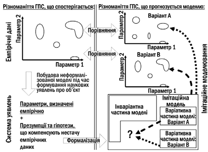
1.7. Testing Hypotheses Reflected in the Variable Part of the Model As has already been noted, a model makes it possible to analyse the results of the simultaneous action of an entire "bouquet" of intertwined chains of causal relationships. In solving this class of problems, our system of thinking and our logic frequently produce errors. At the same time, even a simple algorithm of a simulation model is capable of "unwinding" what we cannot effectively operate with in our own minds. Once the model is launched, it may exhibit inadequate behaviour related to the fact that some of the assumptions used in its construction contradict one another. In such a case, as noted in the preceding section, the realisation of a simulation model makes it possible to correct the conceptual model or the general system of conceptions about the original. The capacity of the model to test various assumptions on the basis of which its algorithms were constructed can also be used deliberately. For this purpose, the model's algorithm should be divided into two parts: invariant and variable. The invariant part of the model's algorithm is realised in any case, since it reflects those features of the original that can be considered reliably established. The variable part of the algorithm can be represented by several alternative variants, each of which reflects a certain hypothesis about the unknown aspects of the functioning of the original system. How will the contradiction between a certain hypothesis reflected in one of the variants of the variable part of the model, and reliably established facts, manifest itself? Not only in the inadequacy of the model's operation. The results of modelling can be tested for correspondence with the results of observations of the original system. Here is how this process was described in a paper devoted to modelling the diversity of HPS (hemiclonal population systems) of the hybridogenetic complex of green frogs (Fig. 1.3). Fig. 1.3.