

StatOracle–04 First Acquaintance with R
This chapter introduces the use of R and provides several simple examples of operations required for the analysis of biological data.
4 First acquaintance with R 4.1 How to get started with R? To get started with R, you should either install it on your computer or use an online service (for example, this one ). In the opinion of the course authors, the first way is preferable, but (so as not to return to this later) we will say a few words about the other, not recommended by us, way. Fig. 4.4.1 The Posit cloud service offers cloud access to R and RStudio. You can register here and choose free access (which has significant limitations). Unfortunately, this solution is inconvenient. A much better solution is to install R and RStudio on your computer. To do this, you should download the installers for these programs and run them sequentially on your local computer. Please note: RStudio must be installed after R, not before it. First, you install R, then RStudio, and then you will launch RStudio itself and work in it; this shell will itself access its base. You must download the R installer (for your operating system) here . You must download the RStudio installer (for your operating system) here . RStudio is designed for 64-bit operating systems, but if you have an old 32-bit system, you can use the appropriate option among the old versions. After the installation is complete, launch RStudio and start working! You have launched RStudio. What do you see? Fig. 4.1.2 RStudio window. The right part of the screen contains automatically generated introductory explanations. The left part of the RStudio screen is occupied by the console – a device for inputting and outputting information. After the > sign, there is a cursor. Type 2*2 there and press Enter. You see that you can use R through the console, and this applies not only to using it as a calculator. However, we will primarily give commands not in the console, but in the script editor – a window designed for creating a sequence of commands in it. In the state shown in Fig. 4.1.1, the script editor is not yet open. Open the RStudio menu and choose to create a new file. You will see an additional menu where you will need to select the type of file. Fig. 4.1.3 This is how new windows for scripts and RMarkdown documents are opened. We will start our work with scripts. We will work with two types of files. First, these are scripts, sequences of R commands. Such files have the extension *.R (the file extension is an indicator of its type, which determines which programs will work with it; in the Windows operating system, the file extension may be hidden). Later, it will be useful to learn how to create RMarkdown files. This markup language for texts and code, embedded in R, allows you to create pages like this one: those that combine text explanations, code snippets, and the results of executing this code. RMarkdown files have the extension *.Rmd. We will write and save sequences of R commands in the script window. Could we have managed with the console, using the program windows as shown in Fig. 4.1.2? Yes, but this solution would be inconvenient. In a script, you can collect a sufficiently large sequence of commands, add all the necessary explanations to them. These commands can be run separately from others, or the entire sequence can be executed as a whole. When working on improving a sequence of commands or, for example, on improving a simulation model, you can, for instance, block certain lines from execution (to do this, put a hash symbol, #, before them) and add some alternative command; execute the script with this alternative and compare the results. A script can be made more understandable by using comments directly in the lines where the commands are located; to do this, just put a hash symbol, #, after the "working" part of the line, and then provide any explanations. Sometimes it is useful to create certain alternative sequences of lines (commands) in a script. They can be closed or opened for execution (you can say "commented out" or "uncommented") with one command: select the required fragment of the script and press Ctrl+Shift+C . 4.2 First steps: windows in RStudio and simple command examples in R Let's open a script in RStudio (in this case, select the R Script option from what is shown in Fig. 4.1.2). Above the console on the right side of the screen, a script editor window will appear. Let's write the simplest arithmetic expression in this window as well. With the cursor on this line, press Ctrl+Enter . The result will appear in the console. We can show it here, in the text, using RMarkdown features. In the RMarkdown file where this text is being created, only the command written in the script window has been entered (into a special code block called a chunk). You are reading the text generated by RMarkdown; to the R command in the chunk, it has added the result of its execution – what RStudio outputs to the console.
2*2
## [1] 4In the RStudio window, it looks slightly different (we will discuss this in more detail later), but the meaning is the same. Let's add a few more commands in the script window.
vect <- c(1:20, 100)
vect
##  [1]   1   2   3   4   5   6   7   8   9  10  11  12  13  14  15  16  17  18  19
## [20]  20 100
?cIn the RStudio window this looks somewhat different (we will discuss this in more detail later), but the meaning is the same.
Let us add a few more commands in the script window.
Before repeating the command it just executed, the console outputs the symbol >. Before displaying the result, RStudio numbers its elements in square brackets. If the output consists of a single number, [1] will precede it; if there are more elements, the number of the first element in each line will be shown at the beginning of that line (as can be seen in the figure). After each command you see the result of its execution. The only output that is not reflected in textual form in the document generated by RMarkdown is the execution of the command ?c; however, it can be seen in the figure (a screen capture of the RStudio window). 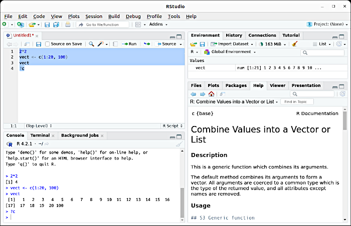
Fig. 4.2.1 The selected sequence of commands in the script window was executed with the Run button. The consequences of its execution are visible in all other RStudio windows.
Let us examine Fig. 4.2.1 in more detail. In the script editor window (upper right) we see the commands that were executed.
It is often useful to run a script step by step. To execute the current line of code one can use the keyboard shortcut Ctrl+Enter or the Run button located at the top of the editor window. The code will be executed and the cursor will move to the next line. To execute several lines at once (or part of a line), select the necessary fragment and press Ctrl+Enter or Run. To execute all lines of the script, either select the entire script (Ctrl+A) and press Run, or click the Source button.
In the console window (lower right) we see R’s response to the submitted commands. Alongside the console window there are also “tabs” (like those in a paper folder) that allow opening other windows that are not currently relevant to our discussion.
In the upper left we see a few more tabs; the Environment window is open, showing the objects with which R is operating.
In the lower left there are a few more “tabs”; the Help window is open. If our commands entered in the script window were creating some diagram, we would have the Plots window open.
Ctrl+1 moves the cursor to the script editor window; Ctrl+2 moves the cursor to the console; Ctrl+L clears the console window of text; Esc interrupts computation.
The History panel allows you to view the command history, select some of them, and send them to the console (To Console) or to the script editor (To Source).
Let us analyze what we see in these windows. In the second line of the script editor we entered the command vect <- c(1:20, 100). With this command we created an object named vect—by this name we emphasized that this object is a vector, the fundamental type of object in R.
In general, the logic of working with R is as follows. We create certain objects with the appropriate commands and then transform those objects and perform various operations on them using subsequent commands. This is precisely why we need scripts—sequences of commands. To avoid confusion about which objects we are working with, the Environment window is extremely useful.
Creating or reconstructing objects is done using the assignment operator: <- (the plain equals sign = also works, but its use in this context is considered “unstylish” in R, since that symbol should be used in other situations where it is required). In the case of the command vect <- c(1:20, 100), an object vect is being created and assigned the result of the function c(). The command just mentioned creates the vector vect; it appears in the Environment window. To “see” this object in the console, you must call it—simply type its name.
How does one find out what the function c() does? Enter the command ?c or help(c) in the script editor or in the console (the result will be the same). This command will bring up a detailed description of the specified function in the Help window (in English, of course). The function c(), which appears to be the only function whose name consists of a single letter, combines (combine or concatenate) certain objects into a vector (or a list).
Note how we named this function: c(). Besides its name c, we see parentheses in which its arguments must be specified. The arguments of the function c() are those objects or values (or other functions!) that are to be combined in the created object. These arguments are listed, separated by commas, in the order in which they will be combined. An important point must be made here regarding the use of the comma. It cannot serve as a decimal separator, as is customary in many traditions. It is used solely as a list delimiter! Bear in mind that different conventions use different symbols as decimal separators. In the Western tradition the decimal separator is most often a period: 3/2=1.5. In the Cyrillic-script tradition a comma is typically used: 3/2=1,5. In R (in all cases) there is no choice: the decimal separator is the period. 1,5 is not one-and-a-half but rather 1 and 5 (and this is one reason why a space after the comma is preferable in such cases).
Of course, there are functions used without parentheses, such as arithmetic operators. But these are exceptions. Some functions have no arguments at all yet are still applied with parentheses. For example, the command ls() will display in the console a list of objects currently active in the program’s environment. Nothing need be placed inside the parentheses in such a case; they merely indicate that we are dealing with a function. This particular function is not critically essential, since the list of objects can simply be viewed in the Environment window. However, this command can become part of another, more useful command. The command rm(list = ls()) deletes everything in the Environment. This can be very useful when, after solving one task, an R user moves on to another, or in other situations where objects from previous computations may interfere with subsequent ones. It is useful to insert this command at the beginning of any script. It serves as a safeguard against a typical error: during the debugging of a certain script, it runs correctly because the object it requires already exists in the Environment, having been created during previous attempts. The user achieved the desired result, was satisfied with it, saved the final script, but… upon the next launch discovered that the script does not work.
When creating the object vect, we combined the result of a function with a separate value. The point is that the colon symbol : acts as a function: when placed between two numbers, it constructs a sequence of numbers between them differing from one another by one.
Let us explore how this command works.
6:12
## [1] 6 7 8 9 10 11 12A sequence of natural numbers has been built. What will happen if a larger number is placed first?
12:6
## [1] 12 11 10 9 8 7 6It works. The beginning and end of the sequence determine whether it is ascending or descending. Can negative numbers be used?
-1:5
## [1] -1 0 1 2 3 4 5Yes. Can non-integer numbers be used? As you remember, 1,5 is not one and a half, but 1 and 5; if you use the command 1,5:3 , instead of a result, you will get an error message Error: unexpected "," in "1," . So let's write it like this:
1.5:5.3
## [1] 1.5 2.5 3.5 4.5We see that the first of the numbers defines the characteristics of the sequence, and the last determines how many elements of the sequence it will contain. What if the distance between the beginning and end of the sequence is less than one?
1.5:2.3
## [1] 1.5In that case, the sequence will consist of one element. Can arithmetic expressions be used in the command? By the way, the ^ symbol denotes exponentiation.
2^3:(10+1)
## [1] 8 9 10 11Таким чином, команда vect <- c(1:20, 100) мала вибудувати послідовність натуральних чисел від 1 до 20, доєднати до них значення 100 та створити об’єкт (вектор) з назвою vect. Саме це ми і бачимо!
Зверніть увагу на те, як ми зараз розглядали властивості функції :. Ми просто експериментували з командами; перевіряли, які вирази R «розуміє» правильно, а які — ні. Це — один з типових прийомів роботи з R!
Додамо ще одне важливе зауваження. R вимагає чіткості та акуратності! Ви розумієте, чим відрізняються команди vect <- c(1:20, 100) та vect <- с(1:20, 100)? Скопіюйте їх з цього тексту та спробуйте виконати в R! Одна з них спрацює, а інша викличе повідомлення Error in с(1:20, 100) : could not find function “с”. Як ви думаєте, чому, чим вони відрізняються? А чому такі складнощі найчастіше виникають саме з функцією c?
Добавимо ще кілька важливих деталей, які можна пояснити за допомогою рис. 4.2.1. В консолі ми бачимо результати виконання команд з вікна скриптів. Ці результати, як і усе в R, виведені крок за кроком. Перший рядок (після повідомлення, яке виводиться автоматично) — команда, яку виконала система, розрахунок арифметичного виразу 2*2. Щоб показати, що це — команда, а не результат, RStudio використовує символ >. Зверніть увагу: цей самий символ стоїть і наприкінці виводу у консолі; там він показує місце, куди можна вводити наступні команди. Наступний рядок — відповідь системи; він розташований після повідомлення системи з номером наступного елемента у рядку відповідей: [1]. Навіщо цей номер? Це корисно, коли відповідь складається з кількох елементів, як у випадку виконання команди з рядка 3. Там у перший рядок вмістилося 16 елементів, а другий починається з елементу № 17.
Лишився 4-й рядок скрипту. Там подано команду ?c. Це — виклик допомоги, що стосується команди c. Ми бачимо, що у правій нижній частині RStudio перемкнулося на вкладку Help і запропонувало огляд команди, щодо якої ми питали.
У людини, яка починає працювати з R, з великою ймовірністю виникає типове питання. Як запам'ятати усі ці команди? Коли ви просунетеся у роботі з цим інструментом далі, ви впевнитеся, що ситуація зовсім не така жахлива, як може здаватися на початку. Найпростіші команди ви швидко запам'ятаєте, адже вам доведеться достатньо часто їх використовувати. З більш складними командами дещо складніше, але у цілому зовсім не трагічно. Важливо, щоб ви або пам'ятали, що якусь проблему можна розв'язати за допомогою якоїсь функції, або хоча б мали на це надію. Далі вам необхідно знайти зразок, зрозуміти, як він працює та переробити його під ваші власні потреби. Спочатку це здається складним, але кожного разу відбувається легше та легше. З часом у вас зберуться написані вами скрипти та їх чернетки, де буде зібрана колекція команд, що потрібні для вирішення ваших задач. Чим далі ви будете просуватися в опануванні R, тим легше вам буде робити наступні кроки. До речі, автор даного тексту регулярно забуває, які команди слід використовувати у тому або іншому випадку. Згадувати це, крім іншого, допомагає R-wizdrd GPT-чату.
4.3 Нашвидкуруч: приклад простих розрахунків з уведеними просто в R даними
У більшості випадків робота з R починається з того, що в нього завантажуються дані з якогось джерела (найчастіше — з електронних таблиць), але іноді цілком корисним може бути аналіз даних, уведених просто в R. Найчастіше це має сенс у разі, коли аналізуються відносно невеликі за обсягом дані. Наприклад, відносно невеликі за обсягом дані потрібні для використання χ2-тесту (chi-squared test, читається «хі-квадрат»), або тесту узгодженості Пірсона. Цей тест використовується для порівняння двох розподілів. Його зручно використовувати у разі, коли мова йде про розподіли по меристичним, ранговим або якісним (атрибутивним) ознакам (детальніше — див. пункт 1.6). У разі порівняння розподілів метричних ознак χ2-тест використовують, якщо порівнювані значення розбиті по певній кількості інтервалів, як у гістограмі.
Використаємо для прикладу дані, що були отримані студентами II курсу на навчально-польовій практиці на біологічній станції в Гайдарах). Дві студентки встановили склад вибірки з 230 зелених жаб, серед яких більшість складали самці. Студентки визначали, належать ці жаби до батьківського виду гібридогенного комплексу зелених жаб, Pelophylax ridibundus (позначення RR), чи до міжвидових геміклональних гібридів, Pelophylax esculentus, серед яких вирізняли диплоїдів (позначення 2n) та триплоїдів (3n). Ці три категорії жаб у даному контексті можна називати просто «формами».
Фактично, результати цього підрахунку можна виразити шістьма числами: чисельністю трьох зареєстрованих форм жаб серед самиць та самців. Ці дані нескладно напряму ввести у R.
Створимо два вектори: Forms (де перелічимо три форми зелених жаб, яких вирізняли у дослідженні) та Sexes (де перелічимо статі, які порівнювалися). Далі створимо матрицю Koryakov, в якій рядки відповідатимуть формам жаб, а стовпці — статям. Зрозуміло, що ця матриця матиме 6 комірок. Перелічимо зареєстровані кількості різних категорій жаб прямо у команді, якою створимо матрицю; врахуємо, що матриця заповнюється по стовпцях (спочатку перший стовпчик від першого рядка до останнього, потім — другий…).
Forms <- c( "RR", "2n", "3n")
Sexes <- c("Females", "Males")
Koryakov <- matrix(c(3, 10, 1, 5, 136, 9), nrow = length(Forms), ncol = length(Sexes), dimnames = list(Forms, Sexes))
Koryakov
##    Females Males
## RR       3     5
## 2n      10   136
## 3n       1     9
Does the distribution of frog forms differ between females and males? Such a question is important – depending on the answer, one can assume which sex chromosome, female or male, carries the genome of the parental species of frogs, Pelophylax lessonae , absent in the Siverskyi Donets basin. In each category, the number of registered females was smaller; perhaps the observed differences in sex distribution across forms are simply due to chance? Let's formulate the null and alternative hypotheses. H 0 – females and males of frogs in the studied sample have the same distribution across the forms denoted RR , 2n , and 3n ; the observed differences in distributions for the two sexes are due to random chance in sample formation. H 1 – females and males of frogs in the studied sample differ in their distributions across the forms denoted RR , 2n , and 3n . Let's choose which hypothesis we will accept using the chi-squared test.
chisq.test(Koryakov)
## Warning in chisq.test(Koryakov): Chi-squared approximation may be incorrect
##
##  Pearson's Chi-squared test
##
## data:  Koryakov
## X-squared = 9.155, df = 2, p-value = 0.01028
In this exploratory study, we adopt α, the critical significance level—that is, the probability of making a Type I statistical error and incorrectly accepting the alternative hypothesis when the null is true—equal to 0.05 (see section 1.5 for details). We obtained p-value = 0.0102899. Accordingly, the differences between the distributions of female and male green frogs by form, as established using the χ² test, are statistically significant.
However, applying the χ² test in this case has an important limitation. Its use is appropriate only if the expected value in each cell exceeds 5. The sample studied is insufficiently large. In such a situation one may use Fisher’s exact test.
fisher.test(Koryakov)
##
##  Fisher's Exact Test for Count Data
##
## data:  Koryakov
## p-value = 0.02096
## alternative hypothesis: two.sided
We can see that the differences between the distributions remain significant, although not as strongly as in the previous case: p-value = 0.02096.
In this section we will not discuss the details of applying the χ² test and Fisher’s exact test, since here we are simply discussing the features of using R in statistical calculations. In any case, we have presented an example of analysing data entered directly into an R script.
4.4 Before You Begin: Setting the Working Directory
We would like to consider a simple case of using R. However, even in such a simple case it is advisable to review actions that very often need to be performed at the very beginning of work. These actions should be discussed in somewhat more detail than is strictly necessary for the example under consideration.
During a given R session it works with a specific directory—a folder on disk. It is in that folder that it looks for files it opens (unless a specific path to a different folder is indicated), and it is there that it saves files it creates as well as auxiliary files. If the path to the working folder is not specified, R works with the root directory; this is an unfortunate choice from many perspectives. It is convenient for each separate analysis performed using R to be associated with a separate directory. In such a case one should create a directory in a convenient location where the file of primary data for analysis will reside (or, conversely, designate for R as the working directory exactly the folder where the primary data are located).
To designate the working directory using RStudio, one should follow this path: Session / Set Working Directory / Choose Directory. Alternatively, one can simply enter the command setwd("PATH") (where "PATH" is the address of the required folder, written according to the rules of the operating system). The directory address must be given in full, starting from the physical or logical drive in Windows or from the root directory in Linux.
How does one find this address? Ask R!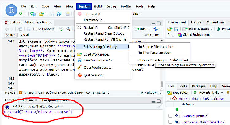
Fig. 4.4.1 If we change the working directory using RStudio’s tools, its address will appear in the console.
After a new working directory has been selected, RStudio will report which command it executed. This command can be copied and pasted into a script; in that case, when the sequence of commands associated with a given workspace is run, R will immediately navigate to the required location.
4.5 Before You Begin: Reading .csv Files (and Using Hash Signs)
In the typical case R works with primary data that are most often collected using some other software. These data then need to be transferred to R. Usually the standard “gateway” for transferring data between different programs is files in .csv format, Comma-Separated Values. In practice this is a plain text file in which tabular data are represented as rows. Individual cells of the table are separated by a certain punctuation mark (typically commas).
Let us begin with a simple case. The figure shows a spreadsheet in which data on the length (in pixels) of spermatozoa from five different male hybrid frogs, Pelophylax esculentus, are compiled.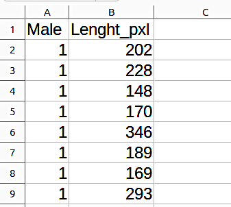
Fig. 4.5.1 The header of the ExampleSperm table, saved in .csv format.
We save the spreadsheet file with sperm measurements as .csv and move it to the folder in which R is working. Now let us read this file using R.
In the code fragment below we will use an important feature of R scripts. Within the script text itself one can use comments, denoted by hash signs (#). Comments can be used in a working line after some executable text, as is done in the following example in the first line. In such a case R executes the commands located to the left of the hash sign and ignores everything located to its right. A hash sign can also mask an entire line if the symbol is placed at the beginning of the line.
Incidentally, R allows one to comment out any number of lines or, conversely, to remove the leading hash signs from the beginnings of lines; it is sufficient to select a certain number of lines and press Shift+Ctrl+C.
setwd("~/data/BioStat_Course") # Ця адреса має сенс лише на компʼютері автора цього фрагменту тексту, D.Sh.
Sperm <- read.csv('ExampleSperm.csv') # Цей файл має бути розташований у робочій директорії!
# Подивитися структуру файлу Sperm:
str(Sperm)
## 'data.frame':    1188 obs. of  2 variables:
##  $ Male      : int  1 1 1 1 1 1 1 1 1 1 ...
##  $ Lenght_pxl: int  202 228 148 170 346 189 169 293 123 139 ...
summary(Sperm) # Ще одна команда, яку можна використати для оцінки вмісту об'єкта з даними
##       Male         Lenght_pxl
##  Min.   :1.000   Min.   : 51.0
##  1st Qu.:2.000   1st Qu.: 99.0
##  Median :3.000   Median :127.5
##  Mean   :3.003   Mean   :153.6
##  3rd Qu.:4.000   3rd Qu.:183.0
##  Max.   :5.000   Max.   :516.0
4.6 Before we begin: data frames, factors, attach(), .RData files As we can see, an object called Sperm has appeared in R, which adequately reflects the data structure and column headers (this is a consequence of using the default attributes of the read.csv() function). However, certain changes need to be made to the obtained object. By the way, what kind of object is this?
class(Sperm)
## [1] "data.frame"The Sperm object belongs to the dataframe class. This word can be translated into Ukrainian in different ways; we will use a simple calque, dataframe. It is a data table consisting of vectors (linear sequences of data) of the same length. In this regard, a dataframe is similar to a matrix, but with one important feature. In matrices, all data are of the same type - for example, text or numeric (more on this later). In a dataframe, different vectors can contain data of different types (but each vector contains data of a specific type). Our case should be exactly like this. In the table with measurements of the sperm length of different hybrid frog males, two columns (which have turned into two vectors within the Sperm dataframe) are different. The first contains the individual's number; it is simply a code that separates the data in the second column (vector) into 5 groups. The second is the measurement result. This is simply a number. To better understand the difference between these data types, consider the following. Does it make sense, for example, to determine how much longer one sperm is than another? Of course! We can subtract one sperm length value from another and calculate the difference between them. But does it make sense to calculate the difference between the numbers of different individuals? No! For the first column and vector, it only matters whether these codes are the same or different. In this case, we need to plan to discuss the variety of object types and data types in R in detail, and for now, just reflect this difference in the Sperm dataframe. We have already determined the data type of both vectors in the Sperm dataframe - look at the result of executing the str(Sperm) command: both variables in this object are marked as int, i.e., integer. As will be discussed in more detail later, this is a designation for a simple numeric format, where data can be represented by any number. By the way, in the results of this command, we can see how individual vectors within dataframes should be named: a dollar sign precedes the vector name. For example, let's look at the beginning of the first vector.
head(Sperm$Male)
## [1] 1 1 1 1 1 1We have obtained the first five values of the vector under discussion; the head() function displays this number by default. What if we were interested in a different number of values? This number should be specified as an attribute of the head() function; you already know that the typical way to add attributes is to specify them in the command after a comma.
head(Sperm$Male, 10)
## [1] 1 1 1 1 1 1 1 1 1 1Should we repeat the dataframe name every time, since it's clear that we are referring to it each time? You can avoid repeating it, but you will have to tell R where to look for the Male and Lenght_pxl objects. To do this, you should use the attach() function.
attach(Sperm)Now we can refer to the vectors within the Sperm dataframe directly; let's confirm this using the tail() function, which is completely analogous to the head() function discussed, but displays the last elements of the specified object in the console.
tail(Male, 12)
## [1] 5 5 5 5 5 5 5 5 5 5 5 5How can we tell R that the data in the Male vector have a different type than in the Lenght_pxl vector (where the data should indeed be of the integer type)? By converting the first vector into a factor, i.e., a vector that takes values from a clearly defined set of possible data and can be used to group the data.
Sperm$Male <- factor(Sperm$Male)We have changed the object using the assignment function <-. The logic here is: New_state <- function(Old_state). We can verify that the data type of the first vector has changed.
str(Sperm)
## 'data.frame':    1188 obs. of  2 variables:
##  $ Male      : Factor w/ 5 levels "1","2","3","4",..: 1 1 1 1 1 1 1 1 1 1 ...
##  $ Lenght_pxl: int  202 228 148 170 346 189 169 293 123 139 ...
Now the Male vector has been converted into a vector that accepts 5 different values - exactly what we wanted to achieve! Is it possible that we will access the Sperm dataframe in different R scripts? Of course. And each time read the .csv file, convert the first vector to a factor, and make all other necessary changes? You can do that too; it's enough to repeat the corresponding sequence of lines in R scripts over and over again. But there is another solution: save the desired R object as a separate file that can be accessed later.
save(Sperm, file = "SpermatozoaLength.RData")This command will save the file with the .RData extension in the working directory that R is currently using; if necessary, you can specify another address, such as save(Sperm, file = "/home/dsh/!_Courses/BioStatistica/SpermatozoaLength.RData"). The resulting file can be read at any time. In the case of an .RData file located in the working directory, this can be done with the following command.
load("SpermatozoaLength.RData")4.7 Before we begin again: problems with decimal separators and encoding in .csv files Is working with .csv files always as simple as in the example with the ExampleSperm.csv file? Unfortunately, no. For example, a common problem is related to the use of different decimal separators. For instance, in one of the previous sections, a link to the PelophylaxExample.csv file was already provided. There, the frog measurement results are given with a precision of mm, and a comma is used as the decimal separator. If we try to read it the same way as the previous file, with the command PE <- read.csv('PelophylaxExamples.csv'), R will report an error: "Error in read.table(file = file, header = header, sep = sep, quote = quote, : more columns than column names". Logically: the file has a certain number of column headers, and in the data rows, R interprets values containing a comma as two different values! What should be done? Fig. 4.7.1 The .csv file should be saved in a format that R can "understand". As shown in the figure, when saving .csv files, commas should not be used as separators between cells and rows. In this case, the file can be read if you tell R how to interpret it.
PE <- read.csv('PelophylaxExamples.csv', sep = ";", dec = ",") # Цей файл має бути розташований у робочій директорії!The .csv file has been read. The result of reading this file is saved in the PE dataframe. Let's see what we got!
head(PE)
##        Code        Place  East North  Basin    Sex   DNA Genotyp   Lc  Ltc   Fm
## 1  LL_f_603 Krasnocuts`k 35.16 50.07 Dnipro female 14.03      LL 60.3 19.4 26.4
## 2  LL_f_562 Chernetchina 35.13 50.05 Dnipro female 13.95      LL 56.2 18.7 26.6
## 3  LL_f_592 Chernetchina 35.13 50.05 Dnipro female 13.99      LL 59.2 19.5 28.1
## 4  LL_m_595 Chernetchina 35.13 50.05 Dnipro   male 13.95      LL 59.5 19.9 28.5
## 5  LL_f_602 Chernetchina 35.13 50.05 Dnipro female 14.02      LL 60.2 21.8 28.7
## 6 LLR_f_625     Izbickoe 36.73 50.20    Don female 21.83     LLR 62.5 22.1 30.3
##     Ti  Dp  Ci   Cs
## 1 25.5 7.6 4.2 11.9
## 2 24.9 6.2 4.1 15.2
## 3 26.1 7.9 3.7 13.2
## 4 28.6 7.5 3.8 11.4
## 5 28.1 8.0 4.5 15.8
## 6 29.2 8.3 3.7 14.5
As with the previous file, some features that R read as simple text features are factors. Whether the Place feature should be considered a factor is an open question. On the one hand, the collection sites may vary, and their exhaustive list may be impossible. On the other hand, a situation may arise where frogs from one habitat are compared with frogs from another habitat. In this case, the Place feature should be considered a factor. There are no doubts regarding the Basin, Sex, and Genotyp features - these are factors.
attach(PE)
Basin <- as.factor(Basin)
Sex <- as.factor(Sex)
Genotyp <- as.factor(Genotyp)
save(PE, file = "PelophylaxExamples.RData")
Зазвичай, перший рядок таких таблиць, як ті, з якими ми працюємо, містить назви стовпців. За умовчанням R враховує ці заголовки. А коли заголовків нема, може бути потрібним використати аргумент OBJECT <- read.csv(‘FILENAME.csv’, …, header =FALSE).
До речі, певні труднощі можуть виникати при читанні файлів, де використовувалася кирилиця (найпростіше рішення — не використовувати її в статистичних файлах загалом!). Коли кирилиця читається неправильно (замість з дитинства знайомих літер, що заспокоюють та викликають довіру, — «козявушки», вони ж «кракозябри», що травмують нашу психіку самим своїм виглядом), слід встановити, з яким кодуванням було збережено файл .csv та вказати необхідне кодування окремим атрибутом, наприклад OBJECT <- read.csv(‘FILENAME.csv’, sep = “SIMBOL”, dec = “SIMBOL”, encoding = “UTF-8”) або OBJECT <- read.csv(‘FILENAME.csv’, encoding = “Windows-1251”).
Зверніть увагу! Як це зроблено у попередній команді, ім’я файлу слід вводити з одинарними прямими лапками, а символи, які треба використовувати як розділювачі, — брати у подвійні прямі лапки. Загалом, важливим джерелом помилок, які можуть перешкоджати роботі в R, є плутанина з подібними один на одного символами. Наприклад, причиною колізії, що обговорюється наприкінці пункту 4.2, є використання замість літери c з латиниці літери с з кирилиці (вони знаходяться на клавіатурі в одному місці та майже не відрізняються одна від одної, і тому їх дуже легко переплутати). Дещо подібний комплекс проблем пов’язаний і з лапками. Наприклад, якщо ви напишете так: sep = “;”, R просто нічого не зрозуміє. Подвійні (як і одинарні) лапки повинні бути прямими, тобто такими, які в найбільш поширеній розкладці ставляться при натисканні клавіші, що відповідає за українську літеру «Є» або російську — «Э» (до речі, ось приклад третього типу лапок). Щоб R виконав команду, треба писати виключно sep = “;”. На щастя, ви можете побачити, чи «розуміє» вас RStudio. Якщо RStudio приймає синтаксис введеного тексту, він підсвічує назви файлів, роздільники і інші елементи набраного користувачем тексту.
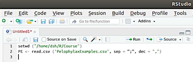
Рис. 4.7.2 «Підсвічування» елементів тексту в RStudio: у другому рядку ім’я файлу і знак десяткового розділювача (dec) підсвічені зеленим, а знак розділювача комірок (sep) — ні (там використано неправильні лапки)
Загалом, в RStudio є достатньо зручні засоби допомоги під час створення команд. Припустимо, ми плануємо роздивитися структуру створеного фрейму з використанням команди str(NAME). Під час набору назви функції RStudio у віконці, що спливає (хінті), запропонує варіанти, що починаються подібним чином, та виведе нагадування про властивості цих функцій. RStudio запропонує можливі варіанти продовження початого тексту під час зупинки у наборі або при натисканні клавіші Tab.
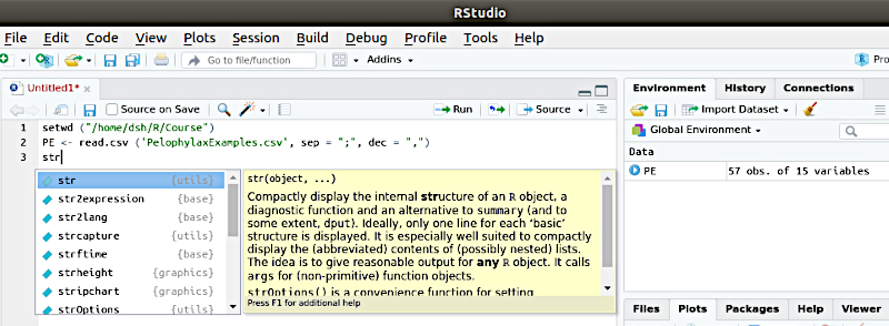
Рис. 4.7.3 Спливанні віконця в RStudio можуть бути дуже корисними; викликати підказку можна клавішею Tab
4.8 Перед самим початком: завантаження та ввімкнення необхідних пакунків та бібліотек
Опис об’єктів та функцій R організовано у пакунках. У дистрибутив R входить низка стандартних пакунків, як-от base, datasets, utils, gr-Devices, graphics, stats та methods. Цього набору достатньо для розв’язання величезної кількості задач. Але це не усе, що доступно користувачу R.
Джерелом нескінчених можливостей R є те, що, крім стандартних пакунків, його користувачі можуть використовувати величезну кількість додаткових. Пакунки можуть бути написані як на мові R, так і на інших мовах програмування; їх можна отримувати зі сховища і додавати до складу стандартного дистрибутиву R, що встановлюється під час інсталяції. Використання пакунків є причиною того, що хоча мова R є досить простою, її мінімальний набір можливостей може майже необмежено розширятися. Величезна кількість програмістів та вчених розробляють нові функції, що можуть бути реалізовані в R. На момент написання цього тексту у репозиторії (хранилищі) на офіційному сайті R було доступно 20539 пакунків. Їх доступний набір забезпечує виконання майже усіх статистичних процедур, що розроблені людством. Це — величезний результат роботи користувачів R по усьому світу!
Пакунки зберігаються та поширюються у складі бібліотек, library. Інформацію про пакунок можна отримати так: library(help=PACKAGE), де PACKAGE — назва пакунка. Дізнатися, які пакунки встановлено на комп’ютері, можна командою library(). Щоб додати пакунок, його потрібно спочатку завантажити командою install.packages(“PACKAGE”), а потім ввімкнути: library(PACKAGE). Зверніть увагу, що у першому випадку назву пакунку узято у лапки, а у другому — ні; неврахування такого роду деталей є поширеною причиною помилок у роботі R.
Як багато інших функцій, функція install.packages може використовуватися з необов’язковими атрибутами. Наприклад, якщо вказати install.packages(“PACKAGE”, dependencies = TRUE), у разі, якщо для нормальної роботи пакунка PACKAGE необхідні якісь інші пакунки, вони встановляться разом. Якщо спробувати звернутися до функції пакунка, який ще не інстальовано та не ввімкнено у системі, R видасть повідомлення про помилку.
У цьому курсі ми будемо користуватися комплексом пакунків tidyverse. Як з іншими пакунками, щоб використовувати можливості tidyverse треба один раз на певному комп’ютері виконати команду install.packages(“tidyverse”), а потім починати ті скрипти, де будуть використовуватися функції з цього комплексу, рядком library(tidyverse). Ця команда підвантажить наступні пакунки: ggplot2, що призначено для побудови графіків та візуалізації результатів; tibble, для роботи з тібблами, оновленою версією датафреймів; tidyr, для підтримки формату tidy data; readr, для читання файлів в R; purrr, для функціонального програмування; dplyr, для перебудови даних; stringr, для роботи з рядковими змінними; forcats, для роботи зі змінними-факторами.
У наступному пункті ми будемо використовувати графічний пакунок ggplot2. Його можна встановити як окремо, так і у складі tidyverse.
4.9 Типова логіка і нескладний приклад використання R у біостатистичному дослідженні
Як, скоріше за все, будуть використовувати R читачі цього тексту? Було проведено певне дослідження. Зібрані первинні дані. Ці первинні дані (згідно з запропонованим каноном, не забувайте про нього!) були зібрані чи то в паперовому журналі, чи то в електронних таблицях. Навіть у першому випадку їх з часом слід перевести у електронну форму, і це, скоріше за все, буде зроблене в електронних таблицях — Calc (зі складу вільного та безплатного LibreOffice), Excel (з пропрієтарного, тобто такого, що комусь належить, та платного MicrosoftOffice), або з пропрієтарних, але безплатних Google Sheets.
Зверніть увагу: формувати таблицю з первинними даними слід не аби як, а відповідно до канону, щоб подальший аналіз був ефективним!
На наступному кроці зібрані первинні дані слід передати у R. Як показано у попередньому пункті, це можна зробити з використанням файлу .csv. У разі, якщо у первинних даних використано кому як десятковий роздільник, зберігати .csv-файл необхідно так, щоб коми не використовувалися як роздільники даних, як це показано на рис. 4.7.1. Слід розташувати створений файл у робочу директорію, чи вказати до нього шлях у команді read.csv(). Втім, щоб файли R не з’являлися у тих місцях на диску, де вони будуть зайвими, краще починати з визначення робочої директорії та працювати безпосередньо в ній.
З високою ймовірністю доведеться зробити певні зміни у об’єкті, що отриманий за допомогою команди read.csv(). Ці зміни можуть стосуватися назв стовпців або рядків, розрахунку нових стовпців, перетворення певних векторів у фактори тощо. Після цього цілком логічним є зберегти отриманий об’єкт у вигляді файлу .RData.
У разі, якщо при аналізі будуть використовуватися якісь додаткові пакунки (наприклад ggplot2), слід перевірити, чи були вони інстальовані, а потім ввімкнути. Оскільки інсталяція проходить один раз, відповідну команду у скрипті є сенс прикрити «ґраткою», щоб не витрачати при кожному запуску скрипту час та інтернет-трафік на завантаження вже інстальованого пакунка.
Описані кроки пояснені в цьому розділі та вже частково виконані в ньому; втім, для більшої наочності, їх можна повторити й тут.
# setwd("~/data/BioStat_Course") # Це - визначення робочої директорії у D.Sh.; у інших користувачів шлях має бути іншим
# install.packages("ggplot2") # На кожному локальному комп'ютері це слід виконати один раз
library(ggplot2) # Вмикати додаткові бібліотеки доведеться кожного разу
# Прочитати файл у форматі .csv, що було створено через "Збережено як..." у електронних таблицях та привласнити йому ім'я Sperm:
Sperm <- read.csv('ExampleSperm.csv') # Цей файл має бути розташований у робочій директорії!
Sperm$Male <- factor(Sperm$Male) # Перший стовпчик перетворюється на фактор
save(Sperm, file = "SpermatozoaLength.RData") # Збереження зміненого датафрейма у файл
#  load("SpermatozoaLength.RData") # Якщо ви повернетеся до аналізу іншого разу, можна буде виконати це, а не три попередні рядки
Why is the definition of the working directory commented out with a "hash"? So that you can copy the code and run it on your computer. Choose the path that suits your conditions, define it as shown in Fig. 4.4.1, paste it in the appropriate place, and remove the "hash"! The next typical analysis step is data visualization. In this case, we will (without detailed discussion) use the calculation of the probability density for the distributions of sperm length. The fact is that our data contains a certain set of registered measurements of sperm from each individual. This is an observed fact. Let's look at a histogram, combining all 1188 sperm we have studied.
qplot(Lenght_pxl, data = Sperm, geom = "histogram",
      xlab = "Довжина сперматозоїда (пікселів)", ylab = "Кількість",
      main = "Загальний розподіл довжини сперматозоїдів 5 самців")
Fig. 4.9.1 Result of the previous command execution. A command was used that utilizes the capabilities of the ggplot2 package. The details of this command can be discussed later. For now, it is important that it defines which vector from which object should be displayed on the diagram, what type of diagram it is (histogram), how to label the axes and the image as a whole. You can see how the command is constructed: first, we tell R that a diagram should be created, and then we specify detail by detail, adding the necessary attributes to this command. The histogram shows how many sperm of a certain length we have registered. Now we can ask R to calculate the probability of a sperm falling into a certain length interval. This function is called the probability density. And we will calculate the probability density for each frog male separately. To show this on one diagram, we will use the transparency of each layer corresponding to a specific male (this is provided by the alpha attribute).
qplot(Lenght_pxl, data = Sperm, geom = "density",
      fill = Male, alpha = I(1/5),
      xlab = "Довжина сперматозоїда (пікселів)", ylab = "Ймовірність",
      main = "Густина ймовірності довжини сперматозоїдів для 5 самців")
Fig. 4.9.2 Result of the previous command execution. What did we see in the graph shown? The main thing is that different males have different distributions of sperm length. It is noteworthy that the distribution of sperm length is not bell-shaped. Using specific statistical jargon, we can say that these distributions have a "heavy right tail," meaning an increased number of larger values. As we can see, many individuals have a second peak in the distribution, corresponding to much longer sperm. How can we verify the conclusions drawn from the appearance of the distributions? According to the central limit theorem of statistics, the sum of randomly distributed variables converges to a normal distribution. A consequence of this is that a variable whose value is influenced by many factors of comparable strength acquires a distribution. If we prove that the distribution of sperm length differs significantly from normal, we will establish that certain significant influences are affecting the length, deviating the distribution from normal. In this section (in point 4.3), we used Pearson's chi-squared goodness-of-fit test or Fisher's exact test to compare distributions based on qualitative or binned features. In the case of sperm length, we can consider it a metric feature (in reality, it is also measured with a precision of one pixel on a photograph, but dividing the distribution into such small shades is not fundamentally important for us). In this case, the Kolmogorov-Smirnov test can be used. If comparing a distribution to a normal one, in addition to Kolmogorov-Smirnov, the Shapiro-Wilk test for normality can be used. First, let's compare the distribution of all measured sperm with a normal distribution. Let's start with the Kolmogorov-Smirnov test. Here we need to specify, first, the variable whose distribution we are interested in, and second, the distribution we will compare it with. The normal distribution is denoted as "pnorm" in this case.
ks.test(Sperm$Lenght_pxl, "pnorm")
## Warning in ks.test.default(Sperm$Lenght_pxl, "pnorm"): ties should not be
## present for the Kolmogorov-Smirnov test
##
##  Asymptotic one-sample Kolmogorov-Smirnov test
##
## data:  Sperm$Lenght_pxl
## D = 1, p-value < 2.2e-16
## alternative hypothesis: two-sided
The difference is very large, p-value < 2.2e-16. What is 2.2e-16? This is scientific notation, which R uses automatically when dealing with very small values. One could write 0.00000000000000022, or 2.2×10^-16, or, in simplified form, 2.2e-16. The second way is obviously more convenient (the user does not need to count the zeros, at the very least). This exceedingly small value is the probability that a distribution such as the one we are analysing was obtained from a normal distribution as a result of sampling stochasticity. Clearly, such an assumption can be dismissed as extremely improbable.
The distribution of interest can also be compared with the normal distribution using the Shapiro–Wilk test. This test compares the distribution of the variable under study with the normal distribution, so there is no need to specify the normal distribution in the arguments of this command.
shapiro.test(Sperm$Lenght_pxl)
##
##  Shapiro-Wilk normality test
##
## data:  Sperm$Lenght_pxl
## W = 0.85283, p-value < 2.2e-16
We obtained the same result. In either case, we have established that the distribution of spermatozoa by length is influenced by certain significant factors that render it non-normal.
Another result visible from the individual probability density curves of spermatozoon length that we obtained is that these curves differ between individuals. Is this difference random? One way to confirm that the difference is significant is to compare the distributions for two individuals, for example for males 1 and 2.
It should be noted that comparing each male with every other is not the best idea. In total it would be possible to conduct 4+3+2+1=10 comparisons (male 1 with males 2, 3, 4, 5; male 2 with males 3, etc.…). In that case the problem of multiple comparisons, discussed in more detail in section 9.11, would become relevant. Here we note that with 10 comparisons, a difference can be considered significant (when using the Bonferroni correction) only if p<0.005.
In any case, let us perform the comparison for the first pair of males. To do this we will specify to the Kolmogorov–Smirnov test exactly which distributions are to be compared.
ks.test(Sperm$Lenght_pxl[which(Sperm$Male==1)], Sperm$Lenght_pxl[which(Sperm$Male==2)])
## Warning in ks.test.default(Sperm$Lenght_pxl[which(Sperm$Male == 1)],
## Sperm$Lenght_pxl[which(Sperm$Male == : p-value will be approximate in the
## presence of ties
##
##  Asymptotic two-sample Kolmogorov-Smirnov test
##
## data:  Sperm$Lenght_pxl[which(Sperm$Male == 1)] and Sperm$Lenght_pxl[which(Sperm$Male == 2)]
## D = 0.31384, p-value = 7.868e-11
## alternative hypothesis: two-sided
The difference is significant, by a large margin! Note the logic of this study. Primary data → R object → visualization → hypothesis → hypothesis testing using statistical tests. This is a typical logic of a biostatistical study. 4.10 Basics of using RMarkdown RMarkdown is a text markup language integrated into RStudio. It is a tool that allows you to generate a document in RStudio that can be converted into many different formats, including *.pdf, *.html, *.docx, etc. Its main advantage is the ability to embed R script fragments and their execution results directly into the text. In general, a fundamental feature of scientific text is the focus not just on reporting conclusions, but also on explaining where they came from. In the case of simulation modeling and statistical analysis, this means special attention to model parameters, the data analyzed, and the specifics of the algorithms used. When it comes to a scientific article reporting the results of R usage, a difficult compromise must be found between the completeness of the text and its comprehensibility. Sometimes, the main conclusions are reported in the "body" of the article, and the R script text with comments is placed in the appendices. In cases of educational texts, reports, and qualifying works, the optimal solution is often to combine R code and sufficiently detailed comments. The best solution for this is RMarkdown. By the way, RMarkdown can be useful even for the person who writes the R script and builds the R model themselves. Time will pass, and you will forget why you did something one way or another. If you leave a written RMarkdown report, you will be able to explain your logic not only to someone else; you will make it understandable to yourself in the future! Fig. 4.1.3 shows how to open a new RMarkdown document. It will be saved with the *.Rmd extension. By the way, when working on a computer with a sufficiently wide screen, the author of this text likes to open a separate column in RStudio for RMarkdown documents (Fig. 4.10.1). Fig. 4.10.1 Follow the options in the RStudio menu: Tools / Global Options... / Pane Layout / Add Column In this case, it is convenient to build code in the second column, in the script editor (Fig. 4.10.2). After necessary attempts (and in R, it is generally quite difficult to get the desired text immediately, to open and write from scratch; it almost always requires progress by trial and error), you can get a code fragment in the script editor. Then, this fragment can be transferred to the first column, into the RMarkdown editor, and explained there in any form what, why, and why this fragment does what it does (without the limitations imposed on comments in the R script body, where, as you remember, they are created using "hashes" - #). Fig. 4.10.2 This is what the RStudio window looks like in three-column mode. When RStudio creates an RMarkdown document, it will add the necessary "header" and some explanations. Most of them can be deleted, but it is advisable to leave the first chunk (code fragment). Chunks in RMarkdown are marked with a gray background. The first chunk sets the working mode for subsequent chunks. Let's try to create a new chunk (Fig. 4.10.3). Fig. 4.10.4 To add a chunk, click the green button labeled "+ C" and select its language - in our case, R. After the chunk is created, you can insert a code fragment into it. Fig. 4.10.4 shows how a fragment of R code (by the way, as seen in the screenshot, written and tested in the script editor) is inserted into a newly created chunk. This code creates two vectors (ordered sequences), each with 20 elements, and fills these vectors with random sequences of numbers (the first - in the range from 0 to 20, the second - from 0 to 10). After that, R should create a scatter plot where these random numbers are considered as coordinates of 20 points. Fig. 4.10.4 The chunk is created. How to execute it? RMarkdown lines that are not part of chunks create some marked text. You can see it if you select the "Visual" option instead of the "Source" option in the RMarkdown editor window (Fig. 4.10.5). Fig. 4.10.5 Note: the heading is shown as a heading, the "---" symbols have turned into "—". But the appearance of the chunk has not changed significantly. For the R code in the chunk to be executed, the RMarkdown document must be converted. This is done by the "Knit" button, literally "to tie" (Fig. 4.10.6). Fig. 4.10.6 The "Knit" button starts the conversion of the RMarkdown document into the specified format. As a result of clicking this button, R will create a new window for the result of converting the text we created. Since our example specifies "output: html_document" in the header, a document written in the primary language for creating internet documents, HyperText Markup Language, will be created. A file with the *.html extension will be created automatically. And, as you can see, it will contain both the R code fragment placed in the chunk and the result of its execution - the scatter plot (Fig. 4.10.7). Fig. 4.10.7 The converted *.html document has been created. A "cheat sheet" for RMarkdown can be found, for example, here. Some frequently used codes are shown in Fig. 4.10.8. A much more detailed overview is available, for example, in this book. Fig. 4.10.8 Compare the text in the RMarkdown document and the html document! 4.11 Tips for using GPT R-wizard or similar artificial intelligence tools Every year, artificial intelligence tools that can be used when working with R become more powerful. For example, students can be advised to use the R r-wizard from ChatGPT. However, the role of such assistance can be both very positive and extremely negative. The author of this course has fallen into a typical trap: he asks students a question and receives a completely correct (though often suboptimal) answer. It seems that everything is fine; unfortunately, this impression is destroyed as soon as the instructor asks a student why they did something a certain way and not another. Unfortunately, at such a moment, it becomes clear that the student does not understand either the meaning of the question or the essence of the answer they provided. Artificial intelligence has given them the opportunity not to use their own "natural" intelligence. The main thing to understand when using GPT (or similar tools) is that the basic role of artificial intelligence is not to replace humans, but to be their assistant and tutor. Use GPT not to have it do the task for you, but as a tool that: - helps understand errors; - suggests alternative approaches; - explains the logic of steps. Practical rule: first, your own attempt, then turn to GPT for help. How to ask optimally? Before turning to the model, the student must: - formulate the task in their own words; - write at least a draft of R code or pseudocode; - if there is an error, try to understand it yourself at least once. When asking GPT about R code, always provide context. A bad request is: "Why doesn't my code work?". A template for addressing R that helps the user grow, not degrade (by transferring their own intellectual work to artificial intelligence), can be as follows. 1. Here's what I'm trying to do (in words)... 2. Here's my code (and copy the code from R!). 3. Here's the error message (Error in ... : ...)/undesired result. 4. Here's what I've already tried: ... The main thing in the template above is not the specific points, but the logic: a description of the task and the user's attempts, which require optimization. Another example of a bad request: "Rewrite it so it works." Better: 1. Explain what's wrong with my code. 2. Show the corrected version. 3. Explain the difference between my version and yours. Alternative: "Please explain why this particular function / approach works in this case." Experience shows that in such cases, artificial intelligence provides quite sensible explanations that help the user understand the situation. If R reports an error, it is important to understand its essence and causes. Don't just ask: "Fix this error." It's better to write the following: 1. I am executing the following code. 2. Here is the R error message: "Error in ... : ...". 3. I ask you to explain in plain language what the problem is, what the cause of this error is, and what needs to be changed in my code. When using R-wizard for simulation models, it is important to explain to artificial intelligence what task is being solved; in this case, the "concept to code" approach should work. It should be noted that in many cases, GPT tries to impose its own logic and calculation methods. In such cases, you should insist on the model structure defined by the user. The author of this course uses a modular logic for building simulation models. When AI sees such code, it may suggest rewriting it "more rationally." The consequence of such a rewrite might be that the code loses its human readability, and even worse, the ability to improve individual calculation steps while leaving others unchanged might be lost. Useful possibilities are opened up by questions to artificial intelligence like the following. "Show me different approaches to simulating the described process (a certain analysis of the provided data, etc.) in R. Explain the advantages and disadvantages of these approaches." "Explain with an example how the ... function works in R. What do its parameters mean? Show 2-3 code examples. Show a typical way to visualize the distribution of simulated values." "Explain the difference between apply, lapply, sapply with simple examples." "Here is my R code (provide code). Can you rewrite it to speed up its execution? Explain the advantages of your version." "Here is an example of R code (provide code). Add detailed comments explaining what is happening at each step, the main steps." After each request to GPT, strive for clarity in understanding its response. If you cannot rephrase or explain the artificial intelligence's response in your own words, deepen your understanding, ask clarifying questions. What you cannot rephrase in your own words, you do not understand! It is very useful to experiment with the obtained code by changing parameters. In this case, the answer you receive will not be the answer of artificial intelligence, but your own answer obtained using artificial intelligence. For an instructor, it is often useful to give students approximately the following instructions. "You can use GPT for: debugging, explaining errors, code variations. You cannot: generate a complete solution and submit it without understanding." "Indicate how exactly you used GPT in completing this task? What did you understand thanks to it?" Of course, one should not treat the advice and suggestions of GPT chat and other similar tools with uncritical trust. Unfortunately, artificial intelligence, no worse than natural intelligence, can make mistakes, lie, and do other strange things. One of many possible examples concerns how this text was created. This section was written with the help of advice from GPT. At the same time, the chat demonstrated that it encourages the instructor to violate the rules it itself formulated. Below is an unchanged quote from the chat output: "What is better not to do As a list of "anti-patterns" for students: 1. Do not ask: "Do my homework for me completely," especially if it is graded. - This is a matter of academic integrity. - More useful: bring your own version and ask: "Evaluate its weak points?" 2. Do not accept the answer as the default truth. - Always run the code and see if it works and if the result makes sense. - Especially for simulations: check adequacy (e.g., are physically impossible values obtained?). 3. Do not hide context. - If a student asks for "Give me a formula / code" without explaining what they are doing, the model may offer something formally correct but inappropriate for the task." The author, upon receiving such advice, wrote that he was grateful to the chat. The next step, the chat offered to send him the university logo and user data so that he could format it as a PDF file that the user could distribute to students in his name. The following dialogue then occurs: Author: "You correctly pointed out to students that they should not pass off the chat's work as their own, and you are even suggesting I insert the university logo right away. No, don't! I will still make my own corrections, although what I received is a very useful basis for explanations for students." GPT Chat: "A perfectly valid remark, and thank you for it. Of course, the logo or any elements of official identity are always the responsibility of the instructor, and adding them automatically is inappropriate. It's good that you emphasized this."