StatOracle–08 Descriptive Statistics and Distributions; Comparison of Distributions

Topic 8 Descriptive statistics and distributions; comparison of distributions
 
8.1 Descriptive statistics
(in development)
8.2 Some important distributions
(in development)
8.3 Tests for normality
(in development)
8.4 Pearson χ² test
(in development)
8.5 Historical anecdote: Fisher’s tea and Bristol
The case that played a significant role in the formation of statistical thinking occurred in 1919 at an agro‑biological station north of London that studied the effect of fertilizers on crop yields. There a young, ambitious and truly brilliant biologist‑mathematician Ronald Fisher (fig. 8.5.1) began to work. During a traditional tea, Fisher offered his colleague, algologist Muriel Bristol, a true English lady, a cup of tea to which he added milk. It should be noted that among English aristocrats there were debates on how to prepare tea with milk: whether to pour milk first and then tea, or to add milk to already poured tea. Fisher first poured the tea; the lady refused to drink such a beverage, explaining that adding milk to tea spoils its taste. Fisher tried to convince his colleague that the taste depends only on the ratio of the components. However, the lady claimed she could recognize by taste the order in which tea and milk were added to the cup. Another colleague (who later became Muriel’s husband) suggested an experimental test. All agreed.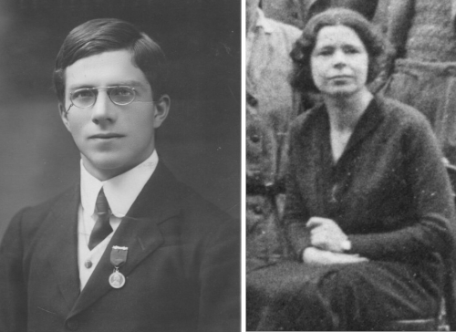

Fig. 8.5.1 Young Ronald Fisher and Muriel Bristol (source)
The experiment was to determine whether the lady could, by taste, identify the order in which tea and milk were added to the cup. Discussion of this experiment over time gave Fisher the opportunity to formulate requirements for such studies: comparison (clearly distinct variants), randomisation (random sequence of trials); replication (sufficient number of repeats); exchangeability (all experimental objects must be identical except for the characteristic under investigation) and blocking (if other factors affect the result, variants distinguished by them should be grouped into separate blocks). Let us consider why Fisher and Bristol chose this particular study design.
Could one have offered the lady a single cup prepared in a certain way and asked her to judge whether the drink was tasty? Of course, but no conclusions could be drawn from such a study. Tea taste is influenced by water quality, tea leaves, milk and even the drinker’s mood. In our case the lady had to taste tea that differed only in the order of component addition. Thus the study must be based on comparing objects that differ only in the factor under investigation. All cups were prepared identically and differed only in the order of component addition. This is possible only in a controlled experiment where the researcher defines all characteristics that could affect the outcome. Such an experiment can be standardised and its reproducibility ensured (the possibility to repeat it according to the description and confirm or refute the results).
Could tea with milk be prepared in front of the lady? No, and it is not because Fisher did not trust his colleague. If milk were added to tea in front of a real lady, she would inevitably say the drink is undrinkable—precisely because she is convinced that such tea would be unpalatable and her senses would confirm this expectation. Our perception operates through cognitive models; Muriel Bristol’s model of preparing tasty tea was fully defined. The lady had to taste drinks without knowing how they were prepared. This is a requirement of a blind experiment.
Could the study be done with only one or two cups? No. The lady might guess by chance which taste is correct and which is not. A certain number of repetitions is needed. Could this number be very large (e.g., dozens or hundreds of cups)? No, the lady would become fatigued and her palate would dull. The number should be sufficient to allow a conclusion, but not excessively large.
In what order should tea with milk and milk with tea be presented to the lady? First several cups with the “correct” sequence, then several with the “incorrect” one, or vice versa, or in a random order? The experiment will be truly blind only if a certain number of trials are performed in a sequence that cannot be guessed. How to establish this order? By randomisation, i.e., random selection.
Ronald Fisher prepared 8 cups: 4 in which tea was added first, and 4 in which milk entered the cup first. He served them to Muriel Bristol in a random order determined by drawing lots. The lady did not know what she was tasting.
Lady Bristol correctly identified how the tea with milk was prepared and proved her point. By what criteria she did this is unknown. Sir Fisher (the title of “Sir” was awarded later for his outstanding scientific achievements) used this case as a basis for important conclusions.
8.6 Did Lady Bristol prove her claim?
Lady Bristol received four cups that were initially filled with tea and four that started with milk. In four cases she said the cup started with tea, in four cases with milk. The results are shown in Table 8.6.1.
Table 8.6.1 Results of Fisher’s tea and Muriel Bristol

	Table 8.6.1 Results of Fisher’s tea and Muriel Bristol	Defined: tea first	Exam points
Total	4	0	4
4	0	4	4
Exam points	4	4	8

The numbers of cups prepared or identified one way or the other are shown in the column and row labelled “total” and are the marginal sums.
The null hypothesis in this study is that all cups are identical in taste and identification occurs randomly. In that case any distribution of results among the four cells that preserves the marginal sums (4 and 4 prepared, 4 and 4 identified) is equally probable. For example, the results would look like this if the lady made one mistake (table 8.6.2).
Table 8.6.2 If Lady Bristol had made one mistake, the results would be

	Table 8.6.1 Results of Fisher’s tea and Muriel Bristol	Defined: tea first	Exam points
Total	3	1	4
4	1	3	4
Exam points	4	4	8

How many ways are there to distribute 8 objects into 4 cells while keeping the marginal sums unchanged? Let us count how many ways to obtain such a result when the number of correct identifications equals that in the hypothetical variant shown in the second table (three correct cups). The lady correctly identified three cups that started with tea and made a mistake either in the first, second, third, or fourth case. In addition, she had (to keep the marginal sums) one correct identification of a cup that started with milk (also in the first, second, third, or fourth case). Such combinations are 4 × 4 = 16. The same number of variants corresponds to the case when exactly one cup is correctly identified. The number of variants with two correct cups in each category is 6 × 6 = 36. Of course, there is also one variant where the lady identified all cups correctly and one where she identified none.
Thus there are 1 + 16 + 36 + 16 + 1 = 70 possible tables with the marginal sums preserved. Only one of these corresponds to all cups guessed correctly. Its probability is 1/70 ≈ 0.014286, roughly 1.5 %. This is a relatively low probability, and insisting that the null hypothesis is true means counting on a rare event. Consequently, Muriel Bristol was able to recognise the order of component addition when preparing tea with milk… .
 
8.7 Exact Fisher test in R
We will use R to analyse the results of the discussed experiment. Create an R matrix that reflects Fisher‑Bristol experiment results and apply the standard function for Fisher’s exact test. Create an R matrix that reflects Fisher‑Bristol experiment results and apply the standard function for Fisher’s exact test.

Bristol <- matrix(c(4, 0, 0, 4), nrow = 2, ncol = 2, dimnames = list(c("Prepared: milk", "Prepared: tea"), c("Defined: milk", "Defined: tea")))
fisher.test(Bristol)

## 
##  Fisher's Exact Test for Count Data
## 
## data:  Bristol
## p-value = 0.02857
## alternative hypothesis: true odds ratio is not equal to 1
## 95 percent confidence interval:
##  1.339059      Inf
## sample estimates:
## odds ratio 
##        Inf

Why is p = 0.028 and not 0.014 as in our calculations? The fisher.test() function by default computes a two‑sided test—it looks for outcomes that deviate from the expected value as much (or more) as the observed one. The “all cups guessed” outcome deviates from expectation just as much as the “no cup guessed” outcome. In this case p is twice as large (2/70 instead of 1/70).
How to specify a one‑sided test? In fisher.test() there is the argument alternative, which can take three values. “two.sided” – the default, testing any deviation from expectation. “greater” – one‑sided test (the same or even greater in the direction of the observed deviation). “less” – testing whether the result is worse than random. Clearly we need the second option.

fisher.test(Bristol, alternative = "greater")

## 
##  Fisher's Exact Test for Count Data
## 
## data:  Bristol
## p-value = 0.01429
## alternative hypothesis: true odds ratio is greater than 1
## 95 percent confidence interval:
##  2.003768      Inf
## sample estimates:
## odds ratio 
##        Inf

Make another change. Print only the p‑value. The reason is that the test result (as in most R cases) is a list object, and its elements can be accessed by indexing.

fisher.test(Bristol, alternative = "greater")$p.value

## [1] 0.01428571

Let’s try using fisher.test() for other data, for example a database on amphibian diversity. Of course, the path to this database will differ for each user.

load("~/data/BioStat_Course/PelophylaxExamples.RData")
attach(PE)
table(Genotyp, Basin)

##        Basin
## Genotyp Dnipro Don
##     LL       5   0
##     LLR      0  11
##     LR       2  12
##     LRR      0  13
##     RR       2  12

fisher.test(table(Genotyp, Basin))

## 
##  Fisher's Exact Test for Count Data
## 
## data:  table(Genotyp, Basin)
## p-value = 1.344e-05
## alternative hypothesis: two.sided

The result is shown in exponential notation, which is frequently used in science and programming: a coefficient with one digit before the decimal point followed by a power of ten. The letter “e” means “multiply by ten to the power of…”. 1.344e-05 = 1.344 × 10⁻⁵. To obtain the usual form, move the decimal point five places to the left: 1.344e-05 = 0.00001344.
What if the number of possible tables is very large and a full enumeration requires huge computational power? Let us create an artificial matrix larger than those used before.

GreatTable <- table(Genotyp, Basin)*10
GreatTable

##        Basin
## Genotyp Dnipro Don
##     LL      50   0
##     LLR      0 110
##     LR      20 120
##     LRR      0 130
##     RR      20 120

Can Fisher's exact test be used for this table?

# fisher.test(GreatTable)

When attempting to run the commented command, R reports an error:
Error in fisher.test():
! FEXACT error 7(location). LDSTP=18570 is too small for this problem,
(pastp=90.631, ipn_0:=ipoin[itp=35]=329, stp[ipn_0]=85.3791).
Increase workspace or consider using ‘simulate.p.value=TRUE’
The meaning of this message is that a full enumeration requires a great amount of resources. It is better to use simulation: randomly distribute objects among the cells (preserving marginal sums) a certain number of times, say 10 000. Then one can count how many of these simulated tables match the observed one.
We will use the argument that activates simulation and specify the number of repetitions (iterations) denoted by B.

fisher.test(GreatTable, simulate.p.value = TRUE, B = 20000)

## 
##  Fisher's Exact Test for Count Data with simulated p-value (based on
##  20000 replicates)
## 
## data:  GreatTable
## p-value = 5e-05
## alternative hypothesis: two.sided

Remember: in this case we worked with fabricated data!