Ecology: Biology of Interaction. VII-04. Some Types of R-Models in Population Ecology: Their Purpose and Structure

As can be inferred from Fig. VII-4.1, one can often distinguish the conceptual model (the design of the simulation model) from its realisation by one or another means. As an example, consider a model implemented in a very simple form — a model in the form of a stack of index cards.
Imagine a set of cardboard cards on which notes can be made in pencil and these notes rewritten when recalculations are performed. There are input cards, on which the input parameters and experimental conditions are written. To simulate random events, we shall use the rolling of dice. The operational algorithm of the model is defined by the sequence, conditions, and rules for recalculating the cards with computed quantities. The working cycle of the model consists of executing such a repeating algorithm and, let us say, moving cards from one stack to another. Of course, when using a model written in R, this algorithm is specified in the model script; in the case of a "card" model, the algorithm may be specified on a certain group of cards indicating which card to proceed to after each step is completed. Incidentally, is it critically necessary for the implementation of such a model to have a stack of cards, a pencil, and an eraser? No. A sheet of paper and a pencil are sufficient, or a surface of wet clay and a stylus for cuneiform writing, or a strip of wet sand on a seashore. In the latter case, one could even learn to rewrite the computed quantities using the time provided by the waves washing up on shore and erasing the previous entries...
Can such models be created? Unquestionably. They could have been created even several centuries ago. Why were they not created, say, in the nineteenth century? Because it was not realised that such models could assist in solving sufficiently complex problems. In practice, such models have a single (but fatal) drawback — they are inconvenient. We can now delegate the repeating calculations, performed according to clearly defined rules, to computers. Incidentally, the variants of realising a conceptual model using a stack of cards, a clay surface for cuneiform, and a sandy shore washed by waves each have particular features; in all likelihood, somewhat different computational algorithms will be optimal for each of these variants. Some of the decisions that must be made when constructing a conceptual model depend on the characteristics of the anticipated means of its realisation.
VII-4.2. Types of Models. Models of Premises and Consequences
We shall not attempt to provide a classification of all possible simulation models; instead, we shall examine several types that are important to us, using population-ecological models as examples. We distinguish educational and research models (notwithstanding the absence of a clear boundary between them). The comparison of arithmetic and geometric growth (see section VII-3) is predominantly educational in character, whereas the model investigating Simpson's paradox in the evolution of altruism (see section VII-5) is research-oriented. The principal differences between these two groups of models lie in their purpose: the former demonstrate well-known phenomena and serve educational purposes, often being illustrative in character; the latter are intended for the acquisition of new knowledge. Nevertheless, there is a continuous transition between typical educational and research models.
Biologists do not always understand how models can be used. In section I-9, the following possible applications of research models are enumerated:
— forecasting the dynamics of a particular process;
— identifying means of control, possibilities for influencing certain processes and phenomena;
— identifying contradictions in ideas about the object of study, refining those ideas (as illustrated in Fig. VII-4.1);
— establishing whether a defined set of causes can give rise to the investigated property of the modelled object.
It can be seen that both relatively applied (directed at solving practical problems) and fundamental (intended for the development of our general understanding of reality) tasks are combined here.
Of particular interest to the authors of this course is the category of models that may be designated as models of premises and consequences. The typical task for such models of causes is to verify the sufficiency of a given set of premises for the emergence of certain properties of biosystems. These models test hypotheses that can be formulated as follows: "Is it indeed the case that the assumptions explicitly proposed during model construction are sufficient to explain certain features of the modelled system as a whole? If sufficient, under what conditions do the proposed causes ensure the emergence of the sought-after feature of the system?" If the model does not exhibit the predicted features, the hypothesis may be considered refuted. When the predicted features do appear in the model, the verification of the adequacy of the assumptions underlying the model's construction may be considered successfully completed. If the investigated properties successfully emerge in the model, can the assumptions about the mechanism of their emergence be considered proven? Can we be certain that the properties of the original system arise in exactly the same manner as they arise in the model? No. A model is not proof, but may serve as an argument. The correspondence between the dynamics of the model and those of the original system may or may not be a consequence of shared mechanisms determining such dynamics. Nevertheless, in accordance with Karl Popper's principle of falsifiability, a discrepancy in such dynamics between model and original can provide the researcher with valuable information about the original system. Successful completion of the correspondence verification between model and original, under conditions in which it was possible to register such a discrepancy, constitutes a step towards improving the cognitive models in use.
Both models of premises and consequences and models of other types may conform to several standard patterns.
Type I models determine the dynamics of a particular process (typically one consisting of a certain number of cycles, each of which comprises several stages) occurring under given initial conditions, parameters, and experimental conditions.
Type II models are meaningful in the case of non-deterministic models in which probabilistic processes are employed. These models establish the probability distribution of simulation results across an ensemble of iterations under identical initial conditions, parameters, and experimental conditions. Such models may be regarded as a means of establishing the results of repeatedly running identical Type I models.
Type III models determine the influence of various combinations of simulation parameters on its outcomes. They are meaningful when one or two variable parameters are used. Such models may be regarded as a means of comparing the results of running a group of Type II models that differ in the parameters employed.
Type IV models enumerate and store in a multidimensional array the results of simulations run with various combinations of key parameters, thereby enabling identification of which combinations correspond to particular simulation outcomes. Such models may be regarded as a means of pre-computing the results of running a series of groups of Type III models that differ in their variable parameters.
VII-4.3. Typical Structure of a Premises-and-Consequences Model Script
Models of the types discussed may have a similar structure; its relatively complete composition comprises 20 functional blocks, combined into five sections. The proposed standard structure of the model is presented in Table VII-4.1.
Table VII-4.1. Typical structural elements of a premises-and-consequences model script

Table VII-4.1. Typical structural elements of a premises-and-consequences model script	HEADLINE: # EXPLANATIONS — EXPLANATIONS: # INITIAL SCRIPT COMMANDS — INITIAL SCRIPT COMMANDS:
E_N_T_R_A_N_C_E	# INITIAL STATE OF THE SYSTEM — INITIAL STATE OF THE SYSTEM: PARAMETERS: # EXPERIMENTAL CONDITIONS — EXPERIMENTAL CONDITIONS: CHANGEABLE PARAMETERS COMBINATIONS:
# W_O_R_K_S_P_A_C_E — W_O_R_K_S_P_A_C_E	# USERS FUNCTION CREATION — CREATING USER-DEFINED FUNCTIONS: CALCULATION RULES DATA: GENERAL OBJECTS CREATION: PARAMETERS COMBINATIONS MECHANISM: ADDITIONAL OBJECTS CREATION:
# W_O_R_K_F_L_O_W — W_O_R_K_F_L_O_W	HIGHER LEVEL CYCLES RUNNING: # INITIAL COMPOSITION CREATION — CREATING THE INITIAL COMPOSITION: # MAIN WORK CYCLE — MAIN WORK CYCLE: ENDING OF HIGHER LEVEL CYCLES:
# F_I_N_I_S_H_I_N_G — F_I_N_I_S_H_I_N_G	# CREATING OBJECTS FOR RESULTS INTEGRATION — CREATING OBJECTS FOR RESULTS INTEGRATION: # RESULTS SAVING — SAVING RESULTS: RESULTS VIEWING: # RESULTS VISUALIZATION — VISUALISING RESULTS:

VII-4. Some Types of R-Models in Population Ecology: Their Purpose and Structure
VII-4.1. Conceptual and Realised Models
The first introduction to simulation modelling was begun in section I-9. Here we shall attempt to make the ideas introduced there more concrete.
Let us draw attention to several circumstances. The creation of a model is a process that may consist of several cycles of refinement and improvement using feedback loops (Fig. VII-4.1). Sometimes substantial progress in understanding the object of study (i.e., in constructing its cognitive model) may be achieved even before its simulation model becomes operational. The formalisation of ideas about the object of study, the identification of key calculated quantities, and the rules for their recalculation can themselves be extraordinarily useful.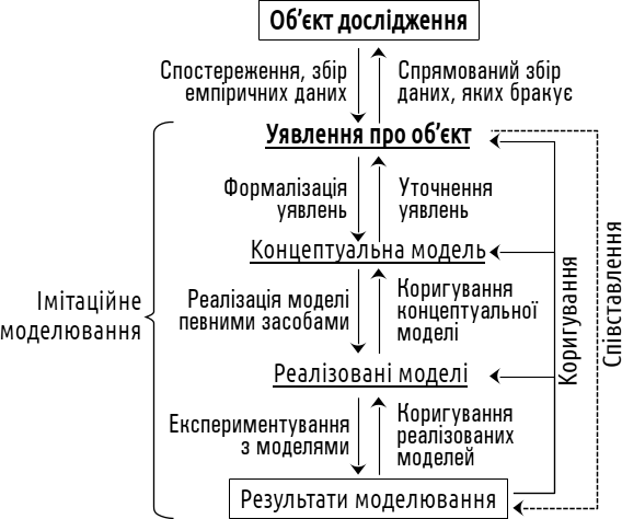

Fig. VII-4.1. Simulation modelling is a process rich in feedback loops that help refine the understanding of the object of study.
When creating a model, one should establish:

What exactly should be observed and investigated using the model?

How should the recalculations of the calculated quantities be structured?

What constitutes the input to the model?

With what set of calculated quantities does the model operate?

According to what rules are recalculations performed during each cycle of model operation?

How exactly will the model be used?

What operating conditions of the model should be chosen?

What are the output data of the model?

How will the output data be presented?

In Table VII-4.1, the names of the structural blocks are written in capital letters (and include colons) because it is in exactly this form that we include them as comments in the text of models written in the R language. The names of the sections and functional blocks of this structure may be indicated in the text of the model script itself to simplify its comprehension and analysis. In the next section (VII-5), examples of a relatively complex model are provided, where one can observe how these labels mark up the text.
What is the purpose of including such additional elements in an R script? A script is a set of commands executed by R, but it is written by a human, understood by a human, and modified by a human. If the script is written correctly, R will "understand" everything required. Enormous problems in working with a model arise when code that is "comprehensible" to R does not correspond to a state convenient for human readers. Even when a particular model is created by a single person, the author of the text will over time forget where and what the model does. For this reason, the script must be well-commented and well-structured. Returning to one's own old model, its author will easily understand where in the script a particular element should be located (for which it is useful to divide the model text into separate blocks), and within the appropriate block — how exactly that code element is implemented (for which detailed comments are useful).
Even more important is the use of dividing the script text into separate blocks when different people work on its text. This is precisely what helps different authors maintain their understanding of the code.
However, the use of the structural elements described above should not become a fetish. These elements are auxiliary tools that help to achieve the primary goal: to create and improve clear and effective models. Of course, not every model requires all the blocks proposed in the structure described in Table VII-4.1. For example, the distinction between the elements "General objects creation" and "Additional objects creation" becomes meaningful in Type III and IV models, where a "Parameters combinations mechanism" appears that conducts groups of iterations with different values of initial parameters. And a section such as "Calculation rules data" is meaningful in cases where tables with the results of crossing different genotypes are used, which may conveniently be created by a separate script and stored as a separate object to be read during model execution. In addition, this structural element is meaningful when using a variable portion of the calculation rules employed to test different assumptions.
VII-4.4. Notation for Stages of the Model Working Cycle
In the model constructed in the preceding section (see subsection VII-3.5), several commands relating to different modelled objects are executed in the working cycle. However, this is a relatively simple model. When it becomes necessary to construct more complex models, their working cycles will often include several stages of calculations, where the results of the preceding stage serve as input to the following one. How should such calculations be organised so as not to become confused by them?
We propose the following solution: to label the stages of calculations within the working cycle using Greek letters.
In some models, a fairly large number of Greek letters must be used. We present the Greek alphabet, from which letters may be copied for insertion into descriptions of what occurs in the working cycle.
α — alpha (al); β — beta (be); γ — gamma (ga); δ — delta (de); ε — epsilon (ep); ζ — zeta (ze); η — eta (et); θ — theta (th); ι — iota (io); κ — kappa (ka); λ — lambda (la); μ — mu (mu); ν — nu (nu); ξ — xi (xi); ο — omicron (oc); π — pi (pi); ρ — rho (rh); ς — sigma (si); τ — tau (ta); υ — upsilon (up); φ — phi (ph); χ — chi (ch); ψ — psi (ps); ω — omega (om).
In addition to the Greek letters and the rules for their pronunciation, we have indicated their two-letter Latin abbreviations. The reason is that while Greek letters can be included in an R script, this will with high probability lead to encoding problems. To avoid potential difficulties, it is simpler to use the abbreviations provided.
Thus, if we denote the population size being reconstructed across several stages as N, then in describing what occurs in the model, we may use the following notation: αN → βN → γN → δN → ωN. Explaining what takes place in the model, we say that on the basis of the alpha-population size the beta-population size is calculated, then the gamma-population size, and subsequently on the basis of the delta-population size the omega-population size is calculated. In the R script, we may in this case use the notations al_N, be_N, ga_N, de_N, and om_N.
The first stage we shall always denote as α, alpha, and the last — regardless of how many separate steps are used in the model — as ω, omega.
"I am Alpha and Omega, the First and the Last, the Beginning and the End."
Revelation of Saint John the Divine, 22:13. The Bible, or the Books of Holy Scripture of the Old and New Testament. Translation by Ivan Ohiienko.
Is this too pompous? Perhaps. But when we engage in simulation modelling, we are in fact engaged in the creation of artificial worlds. To explain this, one may use the introduction to the modelling course given by one of the authors of this textbook, and the ancient Egyptian image (Fig. VII-4.2) mentioned in this "motivational" text.
"The human being is a creature capable of adapting to anticipated environmental changes, which it forecasts through the collaborative construction of models. Knowledge of the world or of oneself, science, art — these are forms of modelling. If you are becoming acquainted with simulation modelling, before all else it is useful to reflect on the wonder of modelling as such.
Why does the sun appear in the sky every morning and disappear every evening? Different answers to this question represent different models. One of the oldest models known to us, approximately five thousand years old, was created in Heliopolis, Egypt. Each morning Nut (the sky) gives birth to Ra (the sun) from Geb (the earth). Each evening Ra disappears into the womb of his mother. Nut and Geb are the children of Shu (air) and Tefnut (moisture). Shu and Tefnut themselves are twin children of Atum, whose name may be understood as "All"; Atum self-organised from the primordial watery chaos — Nun. These deities belong to the Heliopolitan pantheon of primordial gods (Latin primordialis — primeval, pristine), or the Great Ennead. Heliopolis was the centre of the cult of Ra, the Sun. Other cult centres of Egypt created other models and chose other enneads of primordial gods.
Are these fairy-tale, naive explanations? Modern models are more detailed, more mathematised and, above all, provide an effective basis for the scientific-technological transformation of the environment. Mythological models, however, more effectively sustained the spiritual vitality of their users. The ancient Egyptian saw each morning how Nut gave birth to Ra, and this helped him to follow his life's path correctly. Among other things, the adherents of any world-model are concerned with death. The deceased returns to Geb, and, as from Geb, plants grow upward from the body... The users of the Heliopolitan cosmogony placed beside the deceased papyri bearing a text preserved in many variants. It is called the "Book of the Dead," although a better translation of its title is "Chapters of Coming Forth by Day." This text probably did not help one to come forth into the light of day, but it eased the passage into oblivion. The illustrations in such papyri frequently reflected the peace of mind that the mythological model of existence bestowed upon its adherents.
As the symbol of simulation modelling, the author chose an image from the Greenfield Papyrus, which contained the "Book of the Dead" of the queen Nesitanebetashru. We see Shu lifting Nut above Geb, thereby creating the space in which our life unfolds.
Why did the author choose this particular image? It is hoped that students who master modelling will become acquainted with an interesting sensation. Using simple tools, one creates a schematic description of a certain environment... Is it not straightforward to predict how the simulation will unfold? When creating a simulation model of a particular ecological process, one must specify the laws of the imaginary environment and allow it to develop according to the logic one has chosen for it. One runs the model — and sees that it lives its own life, quite often unpredictable, surprising even to its creator. Sometimes the surprises manifest as unfortunate errors and failures; sometimes as counter-intuitive behaviour of the model that reveals something new.
The model begins to live..."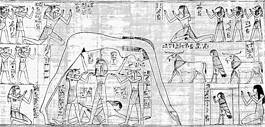

Fig. VII-4.2. This is how the creation of the world was imagined in ancient Egypt. Are our models better?
.