BioStatistics — 02. Topic 2. The Statistica Software Package

Topic 2. Statistical Software Packages and a Sample Data File
2.1. The Diversity of Programs for Statistical Analysis
We have begun studying biological statistics. This study can be organized in two different ways. In the first approach (which may be called "ab ovo"), students are taught the mathematical foundations of the methods under consideration, the necessary formulas are derived, and the theorems that explain them are proved. If a student successfully completes such a course, solving specific problems associated with a given dataset in their field of research turns out to be a manageable task. The second approach ("do as I do") consists of showing students how to solve typical problems using one or another set of tools.
The first approach is more demanding. Those who successfully complete training under the first approach are better prepared and more versatile. However, to a considerable extent, the first approach operates on an all-or-nothing basis. Either you have mastered the fundamental approaches and can apply them, or you do not know what to do and become lost when faced with even the simplest tasks. The second approach is more "democratic" and makes it easy to solve typical problems. Unfortunately, without an understanding of the foundations of the methods, people who have been taught to repeat certain sequences of actions but have not had the meaning of those actions explained to them often make errors. Another disadvantage of the second approach is habituation to particular programs (tools for solving typical problems). Naturally, different categories of students require either the first or the second approach, or a combination of both. Experience teaching biometry to biology students indicates that they predominantly need the "do as I do" approach.
Implementing the "do as I do" approach requires selecting the software packages that will be used for instruction. Here one must choose among five categories of programs:
— free amateur and semi-professional programs; there are many of them, but none are universal, and, moreover, nearly every one requires its own approach (although some solutions deserve recognition as successful, such as this set of online calculators);
— arguably the most successful of the free programs, created by paleontologists as a simplified and free alternative to the Statistica package — the program PAST; the latest version of the program itself and its user manual can be downloaded here;
— free and open-source software; the leader in this area is the R environment: an extremely powerful software package (or language) for statistical analysis (its main page is here); in its basic form it requires working with the command line, although it is more commonly used with interfaces such as RStudio (which can be downloaded here);
— commercial or free software not specifically designed for statistical tasks, but offering broad capabilities for working with data, including statistical analysis; this category includes Excel and Access, components of Microsoft Office, as well as their free alternatives such as LibreOffice Calc;
"One additional point deserves emphasis: under no circumstances is it recommended to perform any statistical analysis in spreadsheet programs. Without even mentioning that the internet is flooded with articles about errors in these programs and/or their statistical modules, it is also ideologically deeply misguided. In other words: Use R!" A.B. Shipunov, E.M. Baldin, "Data Analysis with R".
— commercial professional specialized programs; the market leaders in this area are SPSS and Statistica.
Using programs in the fifth category allows one to focus most fully on the substance of the problems being solved. Unfortunately, this involves the necessity of choosing between purchasing an expensive (very expensive!) license or using cracked, pirated versions. Nevertheless, in the author's view, precisely these programs allow one to acquire the most rapidly the experience of working with data, including through the use of multivariate analysis methods that require highly complex computations.
One of the authors of this manual began working with the Statistica program from StatSoft (in its earlier incarnations) around 1992 (at that time it was called CSS, and it was designed for use in DOS). At that time, this was the program used by qualified zoologists in Moscow and Kyiv. The choice made then determined the program on which the exposition in this manual is based. It must be acknowledged that it is extremely difficult for a person accustomed to working with a program that has a windowed interface, selecting options from a presented list, to transition to working in command-line mode, which requires memorizing the names and syntax of the necessary commands. Nevertheless, there is no longer any alternative to mastering the R environment for a professional biologist.
The authors plan to expand this manual with explanations of how to implement the methods described therein using the PAST program and the R environment. In the meantime, for an introduction to R, one can only recommend the numerous sources available online that describe the use of this package. Among them are blogs devoted to R, including r-analytics and statinr. It is also very useful to take a Russian-language course on working in R.
Online resources devoted to working in Statistica are also available; among them the excellent portal Statosphere deserves special mention.
2.2. Description of the Sample File Pelophylax_example
Powerful tools for data analysis include means for constructing graphs. Very often it is a particular method of visualizing collected data that makes it possible to understand which statistical hypotheses should be tested in the course of further analysis, and to identify interesting or puzzling features of the collected data.
In the exposition that follows, the operational characteristics of the programs will be explained using files that reflect the results of actual research. One such file is the data table Pelophylax_example. For work with this course outline it is recommended to use precisely this file. It can be obtained in one of three ways. First, it can be downloaded (Pelophylax_example.sta) or obtained from the author of this text. When using the electronic version of the course outline, the data presented below can be transferred from the browser window, from a Word file, or from a .pdf file into the required program. Finally, when using the printed version of the course outline, the table presented below can be scanned, entered into the required programs, and then used in subsequent work.
The file uses a fragment of data obtained by A.V. Korshunov in the preparation of his dissertation for the degree of Candidate of Biological Sciences (the author is sincerely grateful to A.V. Korshunov for permission to use the results of his work). The original file contained descriptions of several hundred frogs based on 16 morphometric characters; the selected fragment retains 57 frogs and presents data on variation in 7 morphometric characters in these individuals. The data structure is explained using the Statistica file as an example, because it is precisely this program that allows the most accurate display of text-to-number correspondences and variable specifications.
All individuals described in the sample file belong to the hybridogenetic complex of green frogs, Pelophylax esculentus complex. This comprises two parental species — the pool frog Pelophylax lessonae (Camerano, 1882) and the marsh frog P. ridibundus (Pallas, 1771) — as well as their diploid and triploid hybrids, known as edible frogs, P. esculentus (Linnaeus, 1758). Triploid hybrids of P. esculentus are represented by two forms that differ in genome composition in their genotypes. The reproduction of hybrids is associated with the phenomenon of hemiclonal inheritance. All of the frog forms mentioned may form hemiclonal population systems (HPS), in which both clonal and recombinant genomes are transmitted during joint reproduction.
The parental species and hybrids possess certain external features that, however, do not permit their clear differentiation from one another. One method of evidential identification of the various forms of green frogs involves the use of flow DNA cytometry. Suspended frog cells pass with a flow of liquid through an ultraviolet detector. They are irradiated with ultraviolet radiation at the absorption wavelength of DNA, and the fluorescence intensity (secondary emission) of the cell is then recorded at the wavelength at which the excited DNA emits energy. By comparing the cells of the individuals under study with reference cells (for example, those of the common frog, Rana temporaria), whose DNA mass per cell is precisely known, one can determine the DNA mass in the cells under study. This mass is measured in picograms (pg). Since the genome of P. lessonae is known to have a mass of approximately 7 pg, and the genome of P. ridibundus approximately 8 pg, one can determine from the cellular DNA mass which genomes are included in the genotype of a given individual.
The file Pelophylax_example.sta contains data on frogs with 5 different genotypes. Designating the genome of P. lessonae as L and the genome of P. ridibundus as R, these 5 forms may be denoted as LL, LLR, LR, LRR, and RR. All of these forms occur in the Kharkiv region.
In the file Pelophylax_example.sta, rows (Cases, observations) correspond to individual specimens, and columns (Variables) correspond to their characters. The characterization of each individual includes the collection locality, its coordinates, and an indication of whether that locality belongs to the Dnieper drainage basin (west and northwest of the Kharkiv region) or the Don basin (i.e., the Siverskyi Donets; most of the region's territory). In addition, for each frog its sex is indicated.
The file contains data on sexually mature frogs. When selection was possible, individuals were chosen so that for each frog form the specimens included in the data file originated from different localities.
Measurement of morphometric characters was performed on fixed frogs using vernier calipers; data were measured to the nearest 0.1 mm. The most important of these characters is body length. All other characters may be used either as absolute values or as proportions (the ratio of a given character to body length). In addition, for various purposes one may compute indices — complex characters calculated as certain combinations of the original morphometric characters. Strictly speaking, proportions (ratios of measurements to body length) are also indices, but for convenience these concepts are better narrowed in the manner proposed in this paragraph.
Table 2.2.1. Data included in the file Pelophylax_example
Sexually mature green frogs from the Kharkiv region (non-random sample)

	Place	East	North	Basin	Sex	DNA	Genotyp	L	Ltc	Fm	T	Dp	Ci	Cs
1	Chernetchina	35,13	50,05	Dnieper	female	13,95	LL	562	187	266	249	62	41	152
2	Chernetchina	35,13	50,05	Dnieper	female	13,99	LL	592	195	281	261	79	37	132
3	Chernetchina	35,13	50,05	Dnieper	female	14,02	LL	603	218	287	281	80	45	158
4	Chernetchina	35,13	50,05	Dnieper	male	13,95	LL	595	199	285	286	75	38	114
5	Gorodnee	35,14	50,05	Dnieper	male	16,13	RR	706	266	326	362	97	37	187
6	Krasnocutsk	35,16	50,07	Dnieper	female	14,03	LL	603	194	264	255	76	42	119
7	Gubarevk	35,35	50,16	Dnieper	male	16,27	RR	508	191	259	277	66	27	129
8	Sharovka	35,47	50,04	Dnieper	female	14,91	LR	691	227	359	349	98	48	176
9	Sharovka	35,47	50,04	Dnieper	male	14,94	LR	659	208	302	300	84	48	166
10	V.Gomols	36,27	49,57	Don	male	14,80	LR	553	210	262	280	85	28	144
11	Dobr.yar	36,31	49,56	Don	female	22,60	LRR	715	220	353	344	103	41	155
12	Dobr.yar	36,31	49,56	Don	female	14,95	LR	707	229	334	332	97	43	150
13	Dobr.yar	36,31	49,56	Don	male	14,91	LR	714	244	356	341	93	53	181
14	Dobr.yar	36,31	49,56	Don	female	21,67	LLR	658	241	306	304	96	34	170
15	Dobr.yar	36,31	49,56	Don	male	21,43	LLR	589	216	290	277	77	37	152
16	Liman	36,32	49,35	Don	male	16,20	RR	656	219	352	337	90	36	154
17	Gaydary	36,33	49,62	Don	female	22,79	LRR	742	255	352	356	107	40	174
18	Gaydary	36,33	49,62	Don	female	22,80	LRR	677	294	338	364	108	43	181
19	Gaydary	36,33	49,62	Don	male	22,64	LRR	653	215	315	319	82	38	151
20	Gaydary	36,33	49,62	Don	male	22,81	LRR	691	226	330	334	92	40	167
21	Gaydary	36,33	49,62	Don	male	22,97	LRR	588	206	288	389	91	35	137
22	Gaydary	36,33	49,62	Don	male	22,98	LRR	655	221	328	345	92	45	159
23	Gaydary	36,33	49,62	Don	female	14,88	LR	791	299	381	394	116	47	233
24	S.Gomols	36,34	49,54	Don	female	15,99	RR	535	200	265	281	78	32	145
25	S.Gomols	36,34	49,54	Don	female	22,79	LRR	504	203	231	248	63	31	117
26	S.Gomols	36,34	49,54	Don	female	15,09	LR	877	338	376	423	139	47	227
27	Eschar	36,35	49,47	Don	male	16,03	RR	686	268	336	361	103	38	197
28	Eschar	36,35	49,47	Don	male	14,91	LR	561	209	273	285	77	37	161
29	Lipci	36,38	50,21	Don	female	16,00	RR	701	270	360	376	106	30	178
30	Lipci	36,38	50,21	Don	male	14,86	LR	668	226	335	328	86	44	175
31	Zhovtneve	36,46	50,08	Don	male	16,08	RR	930	265	462	461	138	31	202
32	Zhovtneve	36,46	50,08	Don	female	21,43	LLR	767	240	349	346	95	44	160
33	Zhovtneve	36,46	50,08	Don	female	21,60	LLR	800	262	389	376	116	49	196
34	Balakleya	36,48	49,27	Don	male	15,92	RR	792	262	340	357	93	32	172
35	Balakleya	36,48	49,27	Don	male	22,85	LRR	721	278	359	359	104	47	196
36	Balakleya	36,48	49,27	Don	female	14,85	LR	641	268	317	323	93	41	173
37	Gatishe	36,52	50,18	Don	female	14,91	LR	569	201	260	281	90	36	156
38	PechRibhoz	36,59	49,52	Don	male	14,72	LR	662	252	321	325	92	43	186
39	Izbickoe	36,73	50,20	Don	female	21,83	LLR	625	221	303	292	83	37	145
40	Kreyd.da	36,80	49,43	Don	male	22,73	LRR	755	268	411	372	106	42	189
41	Kreyd.da	36,80	49,43	Don	male	22,74	LRR	564	192	283	293	77	30	139
42	Kreyd.da	36,80	49,43	Don	male	14,79	LR	650	225	320	319	90	38	164
43	Kreyd.da	36,80	49,43	Don	female	21,61	LLR	557	200	251	257	67	33	143
44	Kreyd.da	36,80	49,43	Don	male	21,62	LLR	528	196	257	246	66	31	127
45	Ch.Gusar	36,86	49,41	Don	female	16,07	RR	542	193	262	282	71	27	129
46	Ch.Gusar	36,86	49,41	Don	male	16,01	RR	521	186	243	267	65	28	124
47	Verbun.d	36,89	49,42	Don	female	22,81	LRR	618	212	288	302	94	32	145
48	Verbun.d	36,89	49,42	Don	female	22,85	LRR	689	248	316	341	104	37	179
49	Verbun.d	36,89	49,42	Don	female	14,91	LR	543	190	266	273	79	33	127
50	Verbun.d	36,89	49,42	Don	female	21,50	LLR	616	230	316	298	91	39	155
51	Verbun.d	36,89	49,42	Don	male	21,61	LLR	528	192	258	262	77	35	128
52	Verbun.d	36,89	49,42	Don	male	21,64	LLR	574	199	263	267	78	38	146
53	Martova	36,96	49,93	Don	female	16,18	RR	825	315	423	443	124	49	240
54	Pecheneg	36,99	49,89	Don	female	16,22	RR	537	189	259	273	72	28	119
55	Ch.Shaht.	37,03	49,18	Don	female	22,03	LLR	479	189	238	246	65	27	118
56	Petropol	37,13	49,09	Don	female	16,01	RR	710	256	339	371	99	34	177
57	Veseloe	37,19	49,40	Don	female	16,11	RR	693	247	341	362	104	32	174

To understand the data contained in the file, it is necessary to correlate them with the variable specifications.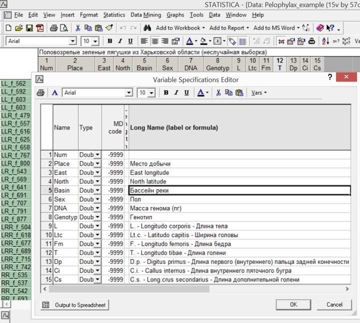

Fig. 2.2.1. Variables in the file Pelophylax_example.sta
The first column in this file contains the designation of the collection locality, the second and third contain the geographic coordinates of that locality, and the fourth contains the designation of the river to whose drainage basin the collection locality belongs. The fifth column presents the sex of the frogs, the sixth the DNA mass per cell (in pg), and the seventh the genotype determined from the DNA mass. Columns eight through fourteen contain the morphometric data (recorded to the nearest 0.1 mm).
Text-to-number correspondences, defined using the text label editor, are assigned to columns 1, 4, 5, and 7. The codes for the first column (collection locality) are of no importance for subsequent analysis, while those for the other three columns merit closer examination.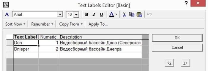

Fig. 2.2.2. Codes for the variable Basin in the file Pelophylax_example.sta
Since the dispersal of frogs occurs mainly along watercourses, the boundary between the Dnieper and Don drainage basins passing through the study area is highly significant from the perspective of the distribution of the various frog forms.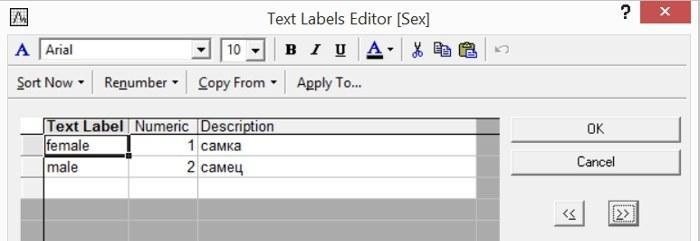

Fig. 2.2.3. Codes for the variable Sex in the file Pelophylax_example.sta
Since the data in this file pertain exclusively to sexually mature frogs, the sex can be determined for all of them. In some cases it is necessary to distinguish juvenile individuals (young animals whose sex cannot be determined) and subadults (semi-adult individuals).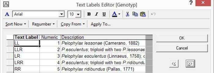

Fig. 2.2.4. Codes for the variable Genotip in the file Pelophylax_example.sta
The variable Genotype divides the frogs into 5 forms under study, each of which is represented by both females and males. The forms LL and RR are "good" species, while the forms LLR, LR, and LRR are interspecific hybrids that bear a name comparable in rank to a species name. In order to avoid complex terminological discussions concerning the status of the frog groups being compared, it is more convenient to call them "forms," treating this concept as a designation for any group of individuals without reference to their taxonomic status.

2.3. The Statistica Software Package
Thus, the Statistica program, produced by the firm StatSoft, offers excellent opportunities for the study of biological statistics. A number of versions of this program are currently available (at the time of writing this text, the latest version is version 13). This program is distributed commercially and is very expensive; pirated, "cracked" versions are currently available. Their use constitutes a violation of the letter of the law, and the decision whether to use such a version is a matter of the conscience of the person making that decision. In addition, versions of Statistica with educational-use licenses have recently appeared. Their existence justifies the detailed description of the use of the Statistica program contained in this manual. It is important to note that this manual deals with instruction in the use of the Statistica program — that is, this manual may be regarded as an advertisement for that program.
Both the original English-language versions of the Statistica program and its various localizations (translations into Russian) are now widely used. It should be noted that the unprofessionally translated Russian-language variants of the program are more difficult to use than the original, even for a person who does not know English. A tenth version of the Statistica program translated into Russian by the Russian representative of the manufacturer, the firm StatSoft, currently exists.
Comments on the installation of the program will not be provided here: any installation package for the program contains instructions on how to do this. Attention should be drawn to an important circumstance relating to the convenience of using the installed program. Statistica can be used not only for research but also for solving serious production tasks (for example, for the formalized processing of client data in banks). For such tasks, the program's ability to assemble into a unified complex the results of different methods of processing a given object may be useful. For this reason, Statistica is capable of generating "workbooks" that bring together into a unified whole all the results of the user's actions.
When investigating biological material, graphs and tables are often generated that do not need to be saved, since the work of a biologist often has an exploratory character. In such a situation it is simpler to output the results of one's work as individual windows.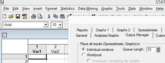

Fig. 2.3.1. To switch the Statistica program to the mode of output in individual windows, navigate to Tools / Options / Output Manager and select the corresponding output option.
Immediately after installation, the program will offer to work with the data-mining tool (DataMiner) or to configure the startup mode. The simplest course of action is to close the startup window and the DataMiner window and proceed to work with data tables.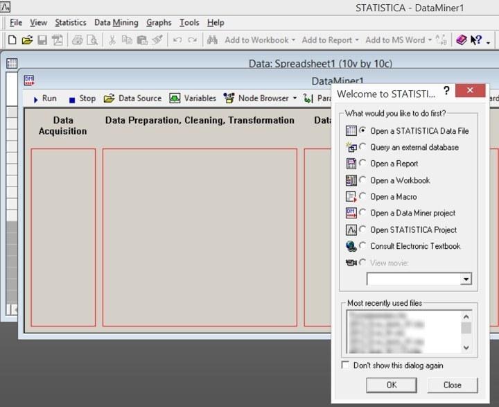

Fig. 2.3.2. Starting work with the Statistica program. For our work we need a window with a data table; the other windows can be closed.

2.4. The Structure of the Statistica Data Table
The data table in the Statistica program is organized in a highly rigid manner: it consists of rows, to which the name of an observation (Cases) is assigned, and columns, which are called variables (Variables). Rows and columns can be added (Add...), moved (Move...), copied (Copy...), and deleted (Delete...).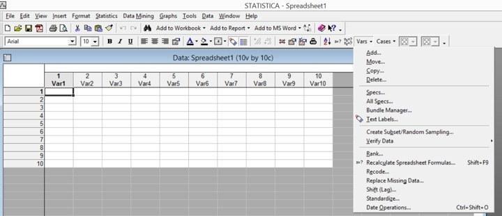

Fig. 2.4.1. The corresponding menu items serve to work with variables and observations (in this case the menu for managing sets of variables, Variables ("Vars"), is highlighted).
When editing data, they are entered into the cells of the table. A single mouse click on a cell will select it; a double-click (or pressing F2 when a cell is selected) will switch it to editing mode. The frame around the selected cell will become thinner, and a cursor will appear inside it. Data can now be entered into the cell.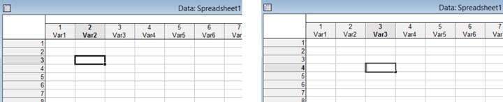

Fig. 2.4.2. The cell on the left in the figure is selected (one or more cells can be selected). The cell on the right is in editing mode; its contents can be modified (for example, data can be added to it).
By pressing the left mouse button and dragging the cursor over the data table, one can select a block — a rectangular region of cells.
Above the column headers there is a field in which the table title can be entered.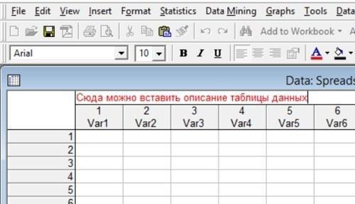

Fig. 2.4.3. Inserting some explanatory notes about the content of the table in its title header can be quite useful.
The very first column of the table contains the names of the observations. A double-click on a name activates its editing mode. An equally important way of managing names consists of using the observation name manager.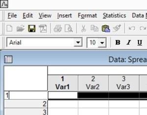

Fig. 2.4.4. Editing observation names.
Looking ahead, it may be noted that in the graphical output of many statistical analyses it is expedient to label the names of observations corresponding to individual objects. It is therefore advisable to ensure that these names are sufficiently short and sufficiently informative.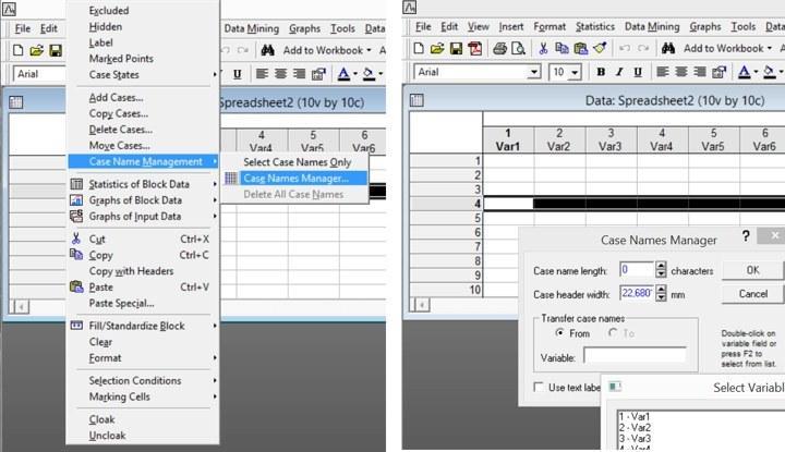

Fig. 2.4.5. To invoke the observation name manager, right-click on an observation name and navigate to Case Name Management / Case Names Manager. Using this manager, one can transfer the contents of a variable to the names, or conversely, create a variable that will contain the observation names. To invoke the list of variables, double-click in the Variable field.
Among other things, the observation name manager can be used to change the width of the window in which the headers are displayed.
For convenience in working with the data table, it is desirable to set the column widths so that column headers and the values entered in the cells fit completely within them, without the columns being excessively wide. This can be done manually by moving the boundaries between columns (between their headers), or it can be done automatically.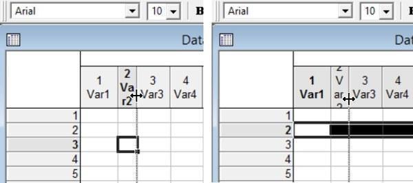

Fig. 2.4.6. A double-click on the boundary between column headers causes their width to be set automatically. In the first case, only one column's width will change (the one to whose right border the click is applied), and in the second, the widths of all selected columns — that is, the entire table — will change.
In some cases it is necessary to restructure the data table by making its rows into columns and its columns into rows (this operation is called transposition). This is done using the command Data / Transpose. This command has two variants: transposing a selected block (which must have the same number of rows and columns) and transposing the entire file (in which the number of columns and rows may differ).

2.5. Operations on Selected Cells in Statistica
Data in selected cells can be moved, and arithmetic progressions defined in adjacent cells can be extended.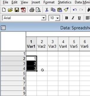

Fig. 2.5.1. A group of cells is selected; the cursor is positioned over other cells and has the appearance of a hollow cross.
When performing these operations, attention should be paid to changes in the shape of the cursor.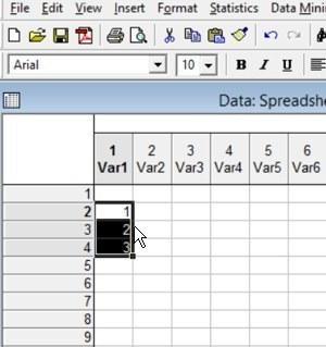

Fig. 2.5.2. The cursor is positioned at the edge of the selected block; performing a double-click in this position and dragging the mouse allows the block of data to be moved to the required location.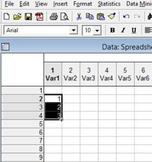

Fig. 2.5.3. The cursor is positioned at the lower right corner of the selected block; performing a double-click in this position and dragging the mouse allows the arithmetic progression defined in the block to be extended to adjacent cells.
If, during the "stretching" of an arithmetic progression, the area to be filled by the resulting sequence extends beyond the boundaries of the table, the program will ask whether to expand the table to the required size or to limit the progression to the existing cells.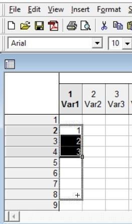

Fig. 2.5.4. "Stretching" an arithmetic progression over several cells.
Finally, it should be noted that by holding down the Ctrl key, one can select several groups of cells that do not necessarily form a rectangular block.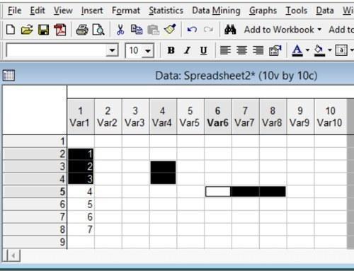

Fig. 2.5.5. To select cells in this manner, it is necessary to hold down the Ctrl key.
A variety of operations can be performed on the selected block, including deleting the contents of cells or performing find-and-replace within them.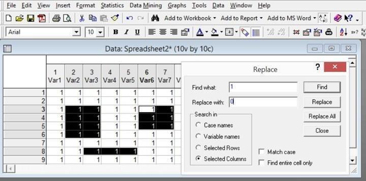

Fig. 2.5.6. To perform a find-and-replace operation, navigate to Edit / Replace, press Ctrl+H, or click the corresponding button on the toolbar (in the figure this button is shown as pressed; it is located near the upper right corner of the figure).
Find-and-replace is an effective method for working with large data files, making it possible to avoid repeated execution of routine actions.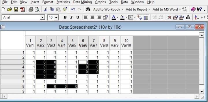

Fig. 2.5.7. The result of the find-and-replace operation shown in the previous figure.

2.6. Working with Rows and Columns in Statistica
The main tools for working with the rows and columns of a data table are found in the default menu items Variables and Cases. The same functions available in these menus are also accessible via the Data option in the program's main menu.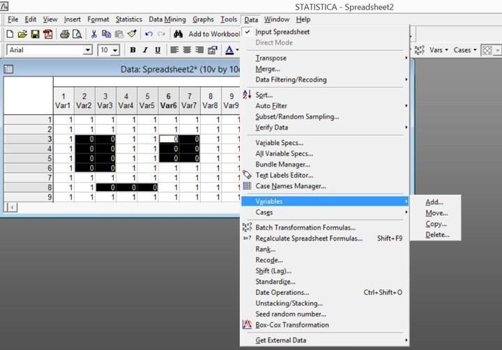

Fig. 2.6.1. Management of columns and rows is available through the Data menu or through the special menus Vars (Variables) and Cases (Observations).
As data are entered into the Statistica table, the need to add columns and rows frequently arises.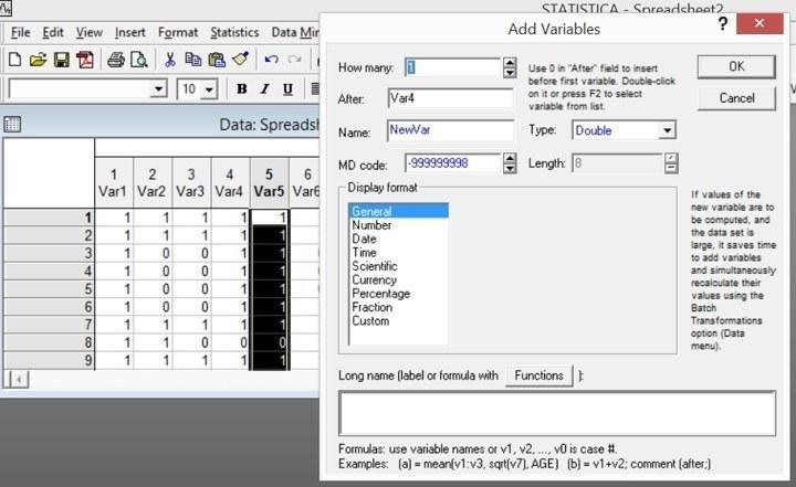

Fig. 2.6.2. When adding variables, Statistica by default proposes to insert them before the column in which the selected cell is located.
When adding columns, one can specify their number, the location at which they are added (after which column), the template for the name (by default NewVar), and certain other parameters that are discussed in more detail later. When moving columns, one can likewise specify which column the group to be moved begins with, which it ends with, and to what location this group of columns should be moved.
The addition of rows (observations) proceeds analogously.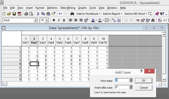

Fig. 2.6.3. When adding rows, they are likewise by default proposed to be inserted before the row in which the selected cell is located.

2.7. Variable Specifications in Statistica
In the Statistica data table, each column has a header above it. The headers are numbered sequentially and by default are named Var 1, Var 2, and so on. To change the properties of a column, double-click on its header.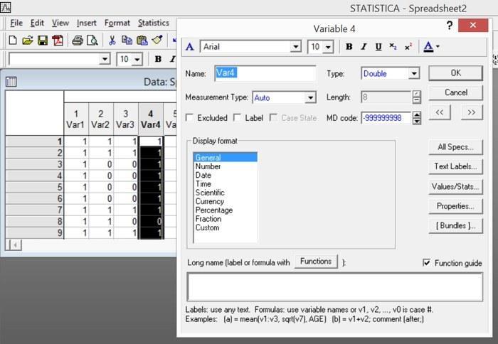

Fig. 2.7.1. Double-clicking on the column header switches to specification mode — editing the variable's properties. Here one can set its name, data type, font, number of displayed decimal places (for numeric mode), a formula for recalculation, and certain other properties.
It is easy to move from one specification to adjacent ones using the arrow buttons located in the upper right part of the dialog box (below the Cancel button). To see the complete list of variables and edit any of them, select the mode Vars / All Specs.... From the specification window of an individual variable, access to the editor is available via the All Specs... button.
In this manual we will not examine in detail the types of variables available in the Statistica program. By default, the double data type is used, which allows both text and numeric data to be stored (this will be discussed in more detail later). In addition, the program provides the option to select a data format. When specifying a numeric format, a window becomes active in which one can indicate to how many decimal places the data displayed on screen should be rounded. There is no need to be concerned about rounding data: the Statistica program will in any case store and use them in calculations at their full extent, with high precision, but for visual perception of data it is simpler to present them in rounded form.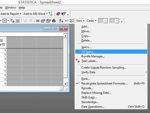

Fig. 2.7.2. Opening the variable specification editor.
First and foremost, students should learn to work with variable names and with the formulas for computing them.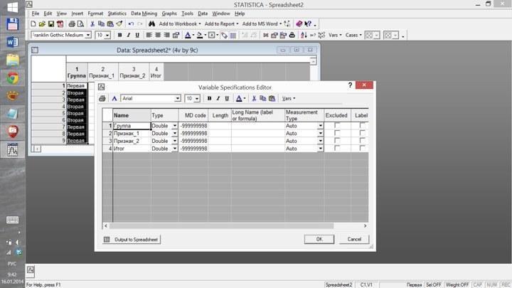

Fig. 2.7.3. The variable specification editor.

2.8. Numeric and Text Forms of Data in Statistica
Data entered into the cells of a data table may have either a numeric or a text form. In the mode in which the comma is the decimal separator, the expression "1,1" will be interpreted as a number (one and one tenth), while "1.1" will be interpreted as text.
Data in Statistica can be of different types. In the default type — the double data type — every text value entered into a given column is assigned a corresponding number. The transition from the display of text data to the display of numeric data can be made by checking or unchecking the box next to the item Display Text Labels in the View menu.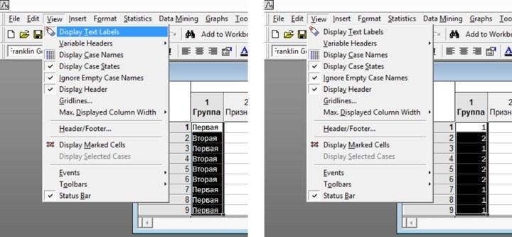

Fig. 2.8.1. In Statistica, it is possible to switch between text and numeric display of data: View / Display Text Labels. In these figures, the difference in display is visible for the variable Group.
The correspondence between text and numeric values is defined in the text label editor (Text Labels...), which for a specific column can be invoked by navigating to Vars / Text Labels..., or called from the variable specification window, as shown in the figure.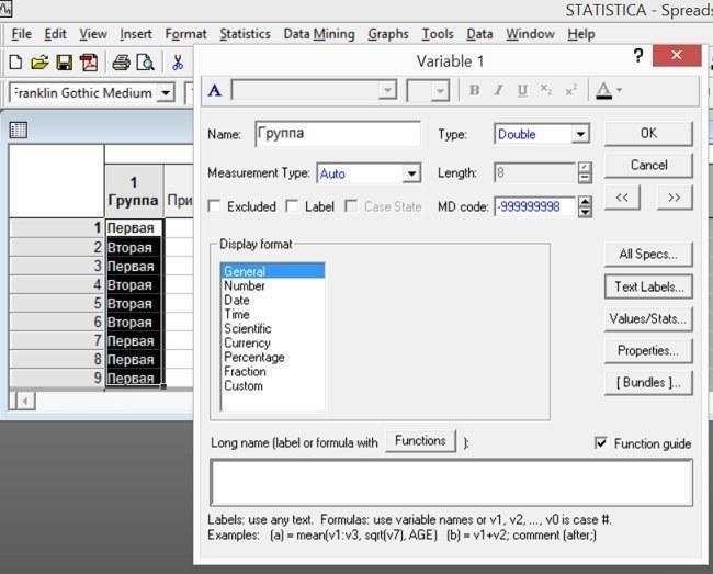

Fig. 2.8.2. A double-click on the header of the first variable (i.e., on the label "1 Group") invoked the variable specification window. In this window there is a button for accessing the text label editor for this variable: Text Labels....
By default, a new value entered in a given column receives a numeric value of 101, the next one 102, and so on. These correspondences may be changed; in doing so, Statistica will ask whether the existing data should be re-encoded to the new codes. Thus, in the example shown in the figure, text-to-number correspondences are set for the variable Group. Such correspondences facilitate data entry: in the corresponding cell one need not write out the word in full, and it suffices simply to enter a number.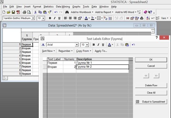

Fig. 2.8.3. The text label editor allows one to define correspondences between text and numeric data. Note the arrow buttons: these can be used to switch to the text label editor for adjacent variables.
Sometimes, during the process of data entry, incorrect text fragments end up in cells. Even if they are subsequently deleted from the data file, they remain in the text label editor together with their numeric correspondences, accumulating there as unwanted clutter. Such unused entries should be deleted (select them and press the Delete Row button).
In the course of using the program, one may encounter problems with the incorrect display of Cyrillic fonts. One universal recommendation is to use the Latin alphabet (for example, writing all names and designations in English). If one wishes to use Russian, display problems may arise.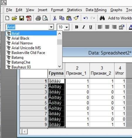

Fig. 2.8.4. An example of the incorrect display of Cyrillic characters (so-called character encoding artifacts).
Such problems can be resolved by selecting a font that displays correctly.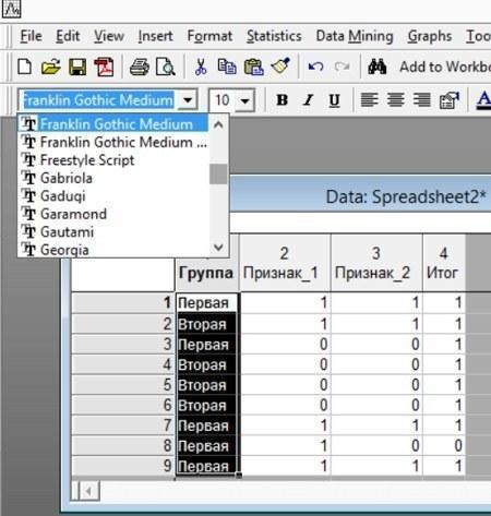

Fig. 2.8.5. With this font, Russian-language text displays as expected.

2.9. Formulas for Data Recalculation in Statistica
In the lower part of the variable specification window (or in the right part of the variable specification editor), one can define formulas by which data are recalculated. A formula begins with the "=" sign, which indicates that the given variable should be recalculated. Formulas use arithmetic signs (+, -, *, /), the exponentiation sign (** or ^), parentheses, and abbreviated designations of various functions. Hints concerning the syntax of these designations appear in pop-up windows (tooltips).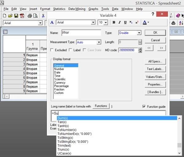

Fig. 2.9.1. If the Function guide checkbox is checked, the Statistica program will offer hints as formulas are entered in the variable specification window.
In formulas, one can use the designations of other variables. They may be denoted either by specifying their names or by designating them by their numbers following the letter "v" (an abbreviation of "variable"), for example v1 or v 15.
Formulas may include logical conditions. These are expressions enclosed in parentheses that contain inside them the "=" symbol or the signs ">" (greater than), "<" (less than), ">=" (greater than or equal to), "<=" (less than or equal to). For example, a variable whose formula field contains =(v1=10) will take the value 1 if variable 1 equals 10 (a true logical condition is considered equal to one) or 0 if variable 1 does not equal 10 (a false logical condition is considered equal to zero).
An expression that will assign the value 1 to a variable when the variable Number is less than 10, and the value 2 when the variable Number is greater than or equal to 10, may look as follows: =(Number<10)+(Number>=10)*2. As can be verified, this formula contains two logical conditions. If the variable Number is less than 10, the first term equals 1 and the second equals 0; if the corresponding variable is greater than or equal to 10, the first term equals 0 and the second equals 2.
When specifying formulas for variables, it is useful to accompany them with comments that will facilitate understanding of what those formulas are for.
In the event that a formula is written in accordance with the rules and refers to variables that exist in the file, when the variable specification window is closed Statistica will offer to recalculate the variable. The calculation will be performed only for those rows in which the cells used by the formula contain some data.
Variables can be recalculated at any required moment using the command Vars / Recalculate Spreadsheet Formulas..., the keyboard shortcut Shift+F9, or by clicking the corresponding button.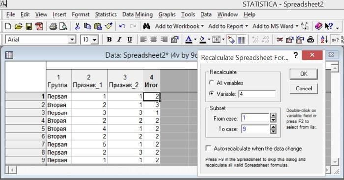

Fig. 2.9.2. The data recalculation window. The cursor points to the button that invokes it (upper left, shown as pressed). Note the option Auto-recalculate when the data change.
In some cases it is convenient to enable the mode of automatic recalculation when data change. In this case, as soon as the contents of any one cell are changed, all other values that use that changed value will be automatically recalculated. However, this mode is not always convenient. For example, when it is active, the undo mode (reverting the last change), invoked by the commands Edit / Undo..., Ctrl+Z, or the corresponding button, cancels not the changes made by the user but the results of the recalculation.
When working with formulas, it should be borne in mind that cells containing no data actually contain a specific number — the missing data code. By default, this number is equal to -9999, but it can be changed in the variable specification window or the variable specification editor. Most of the functions used in formulas operate only on cells that contain data other than the missing data code. Cells whose contents are recalculated by formulas that refer to missing data will also have the missing data code inserted into them. For formulas operating on columns that contain missing data, it may be useful to employ logical conditions such as IsMD(v1), which takes the value 1 if the corresponding variable has no data in a given row (more precisely, if the missing data code is present there), and the value 0 when data are present in the corresponding cell.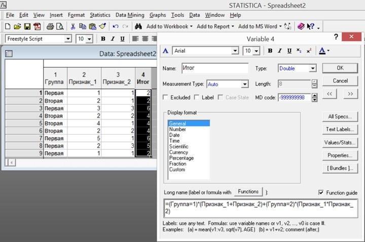

Fig. 2.9.3. For the variable "Total" a formula has been entered that calculates the sum of the variables "Feature_1" and "Feature_2" for objects (rows) from the first group, and the product of these features for objects from the second group. For the formula to work, it is necessary that the first group be assigned the code 1 in the text label editor, and the second group the code 2. The example given is not ideal, as it uses Russian-language names for variables.
In cases where one is working with a file over an extended period, it is inadvisable to refer to variables by their numbers (for example, as v 15). Adding, deleting, or moving variables (whose complete list, it will be recalled, is accessible from the All Specs menu) will change their numbering and disrupt the operation of the formulas that use them. It is better to specify variable names in formulas. This gives rise to recommendations concerning how variables should be named. Spaces and arithmetic signs are undesirable in variable names. If one very much wishes to use a space in a variable name, it is better to replace it with an underscore (_). If these rules are nonetheless violated, the variable name in the formula can be enclosed in single quotation marks, but this constitutes an additional complication of the formula that increases the chances of becoming confused when writing it, and especially when searching for errors in a formula that is not working as desired.