Ecology: The Biology of Interactions. Appendix VII. Semi-finished Components for Building R Models
The idea behind this page is simple: to collect fragments of R scripts that may be useful when creating new models. What should these fragments be called? Examples? Samples? Templates? "Blanks"? Recipes? Let them be called "semi-finished components", semifinished. The content of this page is ongoing; many things in this work remain unclear (for example, it is not easy to decide in what order to arrange these semi-finished components). Nevertheless, we hope that the result of this work will be us
Appendix VII. Semifinished products for creating R-models The idea behind this page is simple: to collect fragments of R scripts on it that can be useful when creating new models. What to call these fragments? Examples? Samples? Templates? "Blanks"? Recipes? Let's call them "semifinished products", semifinished. The content of this page is ongoing; much remains unclear in this work (for example, it is not easy to decide in what order to arrange these semifinished products). However, we hope that the result of this work will be useful for students learning this course. Currently, the following semifinished products are available: Getting started Typical model structure Initial script commands Reading and writing a data file Creating and transforming objects Creating an empty vector of a specific length Creating an empty matrix with named rows and columns Sorting rows in a matrix by the values of a specific column Obtaining parameters of specific categories of individuals from a table with codes; user-defined function Creating a group of random numbers Simulating random events Probabilistic rounding Forming a random sample using the sample() function Modeling selection using the sample() function and a "fate vector" Custom function for competitive population reduction (simulation at the group level) Population reduction due to selection (simulation at the individual level) Non-competitive simulation of population reduction (simulation at the individual level) Competitive reduction of the population from different forms of individuals Calculation management Switch for multiple choice: switch() Iterating through initial parameter values Outputting progress reports to the console Elements of statistics Calculating the correlation between two traits Visualizing results Creating a simple scatter plot Scatter plot with a regression line Creating a line chart for three variables Correlation "heatmap" for many traits Three-dimensional visualization of parameter sweep results Model examples Competition of two clones in a logistically growing population Competition of two species according to the Lotka-Volterra model (in logistic form) with a reaction lag Comparison (and "race") of arithmetic and geometric growth Getting started Typical model structure Most models do not need to use all the listed structural elements, but a certain part of them will be useful. This structure is not a dogma, but adhering to it (at least approximately) and using the proposed subsections in the script text will improve the understanding of the models by users who have mastered it. # I_N_I_T_I_A_L_I_Z_A_T_I_O_N — I _ N _ I _ T _ I _ A _ L _ I _ Z _ A _ T _ I _ O _ N, I N I T I A L C O M M A N D S # HEADLINE — TITLE: # EXPLANATIONS — EXPLANATIONS: # INITIAL SCRIPT COMMANDS — INITIAL SCRIPT COMMANDS: # E_N_T_R_A_N_C_E — E _ N _ T _ R _ A _ N _ C _ E _ C _ O _ M _ M _ A _ N _ D _ S # MAIN PARAMETERS — MAIN PARAMETERS: # EXPERIMENTAL CONDITIONS — EXPERIMENTAL CONDITIONS: # CHANGEABLE PARAMETERS COMBINATIONS IN TYPE III MODELS — CHANGEABLE PARAMETERS COMBINATIONS IN TYPE III MODELS: # R_U_L_E_S_S_E_T_U_P — R _ U _ L _ E _ S _ S _ E _ T _ U _ P # CREATING A SYMBOLS / PARAMETERS TABLE — CREATING A SYMBOLS / PARAMETERS TABLE: # ADJUSTING THE SYMBOLS / PARAMETERS TABLE — ADJUSTING THE SYMBOLS / PARAMETERS TABLE: # CREATING A PARENTS / OFFSPRING TABLE — CREATING A PARENTS / OFFSPRING TABLE: # ADJUSTING THE PARENTS / OFFSPRING TABLE — ADJUSTING THE PARENTS / OFFSPRING TABLE: # W_O_R_K_S_P_A_C_E — W _ O _ R _ K _ S _ P _ A _ C _ E # GENERAL OBJECTS CREATION — GENERAL OBJECTS CREATION: # INITIAL STATE OF THE SYSTEM — INITIAL STATE OF THE SYSTEM: # USERS FUNCTION CREATION — USERS FUNCTION CREATION: # PARAMETERS COMBINATIONS MECHANISM IN TYPE III MODELS — PARAMETERS COMBINATIONS MECHANISM IN TYPE III MODELS: # ADDITIONAL OBJECTS CREATION — ADDITIONAL OBJECTS CREATION: # W_O_R_K_F_L_O_W — W _ O _ R _ K _ F _ L _ O _ W # HIGHER LEVEL CYCLES RUNNING IN TYPES II & III MODELS — HIGHER LEVEL CYCLES RUNNING IN TYPES II & III MODELS: # INITIAL COMPOSITION CREATION — INITIAL COMPOSITION CREATION: # MAIN WORK CYCLE — MAIN WORK CYCLE: # Alpha-composition of the modeled system — Alpha-composition of the modeled system: # Beta-composition of the modeled system — Beta-composition of the modeled system: # Gamma-composition of the modeled system — Gamma-composition of the modeled system: # ... # Omega-composition of the modelled system — Omega-composition of the modelled system: # ENDING OF HIGHER LEVEL CYCLES — ENDING OF HIGHER LEVEL CYCLES: # F_I_N_I_S_H_I_N_G — F _ I _ N _ I _ S _ H _ I _ N _ G # CREATING OBJECTS FOR RESULTS INTEGRATION — CREATING OBJECTS FOR RESULTS INTEGRATION: # RESULTS SAVING — RESULTS SAVING: # RESULTS VIEWING — RESULTS VIEWING (IN CONSOLE): # RESULTS VISUALIZATION — RESULTS VISUALIZATION: Initial script commands The following commands may be useful at the beginning of any model
# Code page UTF-8 + Soft Wrap Long Line in the Code menu in RSudio !!!
setwd("~/data") # Робоча директорія (лише на комп'ютері Д.Ш.!!!)
rm(list = ls()) # Очищення середовища від збережених об'єктів (щоб попередні сесії роботи не заважали наступним)
The first line contains a warning about which code page should be used when opening a specific script in RStudio. If the script is opened using a different code page, Cyrillic characters will be displayed incorrectly. In such a case, the script should be "reopened". In RStudio, this is done using the menu item File / Reopen with Encoding. Additionally, it is convenient to use a mode where long lines wrap to fit the screen. In RStudio, this can be achieved using the menu item Code / Soft Wrap Long Line. Next, it is useful to define the working directory address. To understand which address to use, in RStudio, you can go to Session / Set Working Directory / Choose Directory. When this command is executed using the menu, its correct syntax will appear in the console, which can then be copied to the desired location in the script. The example provided contains the address used by one of the authors of this textbook. Deleting objects contained in the Environment at the beginning of the script is very useful and helps prevent many errors. Reading and writing data files Statistical research in R practically always begins with loading a data file; this step is not mandatory for modeling but can also be used. The first line of the provided script sets the working directory (this is where R will look for and create files). The address used by the author for this course is given as an example; of course, this address will be different for everyone else (by the way, addresses for Windows are structured differently than for Linux). To suggest a data file in \*.csv format to R, it should be created in spreadsheet software (Excel, Calc, etc.). If a comma is used as the decimal separator (as is common on most computers in Ukraine), this should be explicitly stated.
setwd("~/!_Courses/Sex_on_R") # Робоча директорія (лише на комп'ютері Д.Ш.!!!)
Sam <- read.csv('Sample.csv', sep = ";", dec = ",") # Дані перенесені у об'єкт R
summary(Sam) # На створений об'єкт можна подивитися; ця команда виводить характеристики його стовпців
##        X1              X2              X3              X4
##  Min.   : 2.00   Min.   : 3.00   Min.   : 4.00   Min.   : 5.00
##  1st Qu.: 5.25   1st Qu.: 6.25   1st Qu.: 7.25   1st Qu.: 8.25
##  Median : 8.50   Median : 9.50   Median :10.50   Median :11.50
##  Mean   : 8.50   Mean   : 9.50   Mean   :10.50   Mean   :11.50
##  3rd Qu.:11.75   3rd Qu.:12.75   3rd Qu.:13.75   3rd Qu.:14.75
##  Max.   :15.00   Max.   :16.00   Max.   :17.00   Max.   :18.00
##        X5              X6
##  Min.   : 6.00   Min.   : 7.00
##  1st Qu.: 9.25   1st Qu.:10.25
##  Median :12.50   Median :13.50
##  Mean   :12.50   Mean   :13.50
##  3rd Qu.:15.75   3rd Qu.:16.75
##  Max.   :19.00   Max.   :20.00
save(Sam, file = "Sam.RData") # Збереження даних у форматі, що використовує R
load("Sam.RData") # Читання збереженого файлу з робочої директоріїObject Creation and Transformation Creating an empty vector of a specific length
amount <- 10
vect <- rep(NA, amount)
vect
## [1] NA NA NA NA NA NA NA NA NA NACreating an empty matrix with named rows and columns
rws <- c("One", "Two", "Three", "Four", "Five")
cls <- c("First", "Second", "Third", "Fourth", "Fifth", "Sixth")
mtrx <- matrix(NA, nrow = length(rws), ncol = length(cls), dimnames = list(rws, cls))
mtrx
##       First Second Third Fourth Fifth Sixth
## One      NA     NA    NA     NA    NA    NA
## Two      NA     NA    NA     NA    NA    NA
## Three    NA     NA    NA     NA    NA    NA
## Four     NA     NA    NA     NA    NA    NA
## Five     NA     NA    NA     NA    NA    NA
Sorting rows in a matrix by the values of a specific column To begin, let's create a two-column matrix and fill it randomly with numbers from a certain range (more details about the sample() function can be found in the tutorial 'Generating a random sample using the sample() function').
matr <- matrix(sample(1:10, 10), nrow = 5, ncol = 2, byrow = TRUE)
matr
##      [,1] [,2]
## [1,]    4    8
## [2,]    9    2
## [3,]    3    7
## [4,]    1    6
## [5,]    5   10
The byrow attribute ensures that the matrix is filled row by row; without it, it is filled column by column. To sort this matrix by the values of the first column, we will use the given command.
matr[order(matr[, 1]), ]
##      [,1] [,2]
## [1,]    1    6
## [2,]    3    7
## [3,]    4    8
## [4,]    5   10
## [5,]    9    2
By the way, one can make sure that the original matrix has not changed.
matr
##      [,1] [,2]
## [1,]    4    8
## [2,]    9    2
## [3,]    3    7
## [4,]    1    6
## [5,]    5   10
To change the initial matrix, it must be redefined; in this case, the command is enclosed in parentheses, which ensures that the result of its execution is output to the console. Now the matrix matr is sorted.
(matr <- matr[order(matr[, 1]), ])
##      [,1] [,2]
## [1,]    1    6
## [2,]    3    7
## [3,]    4    8
## [4,]    5   10
## [5,]    9    2
Obtaining parameters for specific categories of individuals from a matrix of symbols/parameters. When modeling processes in populations, it is often necessary to specify the values of certain parameters (lifespan, competitiveness, survival rate, fertility, selection pressure, etc.) separately for specific categories of individuals. How can this be done? One option is to use a matrix of symbols/parameters. Let's create such a matrix. Suppose we have 3 groups of individuals (One, Two, Three) characterized by four parameters (A, B, C, D). Let's fill this matrix with some numbers (in a real model, these parameters are set with a specific meaning...).
SP <- matrix(NA, nrow = 3, ncol = 4, dimnames = list(c("One", "Two", "Three"), c("A", "B", "C", "D")))
SP[, ] <- 1:12
SP
##       A B C  D
## One   1 4 7 10
## Two   2 5 8 11
## Three 3 6 9 12
Now, when we need to select characteristics for specific individuals, we can take them from this matrix by simply using a query with the names of rows and columns (of course, enclosing them in quotes to indicate that these are text symbols). If the matrix is filled with numbers, the answer to such a query will be a number.
SP["Two", "C"]
## [1] 8Creating a group of random numbers
mtrx[, 1] <- runif(length(rws), 0, 10)
mtrx[, "Second"] <- runif(length(mtrx[, "Second"]), 1, 2)
mtrx
##          First   Second Third Fourth Fifth Sixth
## One   9.269929 1.072318    NA     NA    NA    NA
## Two   7.516522 1.495302    NA     NA    NA    NA
## Three 5.082234 1.143656    NA     NA    NA    NA
## Four  1.627083 1.769866    NA     NA    NA    NA
## Five  6.134429 1.685893    NA     NA    NA    NA
Simulating random events. Probabilistic rounding. Both the floor() and trunc() functions can be used. A random value uniformly distributed between 0 and 1 is added to the value to be probabilistically rounded; the sum is rounded down (for positive numbers) to the nearest integer. In the example provided, the average of 100 roundings of the value 3.3 should be sufficiently close to this value.
ProbabRound <- rep(NA, 1000)
for (i in 1:1000) {ProbabRound[i] <- floor(3.3 + runif(1))}
mean(ProbabRound)
## [1] 3.296Generating a random sample using the sample() function. The sample(x, size, replace = FALSE, prob = NULL) function can be used both to generate sets of random integers and to select a certain number of objects from a population. The first two arguments are mandatory: x is the range from which the selection is made, and size is the sample size. The next two parameters are optional. If they are not specified, R uses the values provided in the sample full argument record. Thus, the replace parameter determines whether an element that has already been selected can be re-selected. In the case of replace = FALSE, after the first element is selected, the selected value is removed from those that can be selected in the next step. If replace=TRUE is specified, the command will select each subsequent element from the entire population.
sample(1:10, 9)
## [1] 2 9 7 8 4 1 3 6 5
# sample(1:10, 11) # Тут мало б бути повідомлення про помилку
sample(1:10, 11, replace=T) # Тут усе нормально: елементи можна обирати повторно
## [1] 6 2 8 1 9 4 3 1 6 9 7Modeling selection using the sample() function and the "fate vector". The previous example shows a sample use of the sample() function. It can be used to model selection. Assume that the individuals listed in the Al_Pop vector are individuals against which selection s acts. The value of s ranges from 0 (all survive) to 1 (all die). Individuals in whose favor selection works survive completely in this case. Of course, non-competitive mortality, which thins out both types equally, can be as powerful as you like.
s <- sample(2:5, 1) / 10 # Випадково обирається значення добору
s
## [1] 0.4
Al_Pop <- sample(1:100, 12) # Сукупність, яка зазнає дії добору
Al_Pop
## [1] 37 47 56 49 15 27 35 65 74 82 62 4
Fate <- c(rep(NA, s*10), rep(1, (10-s*10))) # Вектор "долі"
Fate # (один на весь скрипт; він не є випадковим)
## [1] NA NA NA NA 1 1 1 1 1 1
Lot <- sample(Fate, length(Al_Pop), replace = T) # Вектор "жереба"
Lot # (створюється окремо для кожного скорочення)
## [1] NA NA NA 1 1 NA 1 NA 1 1 1 NA
Be_Pop <- Al_Pop * Lot # Скорочена сукупність; загиблі - NA
Be_Pop
## [1] NA NA NA 49 15 NA 35 NA 74 82 62 NA
Ga_Pop <- na.omit(Be_Pop) # Остаточно скорочена сукупність
Ga_Pop
## [1] 49 15 35 74 82 62
Custom function for competitive population reduction (group-level simulation). The simulation model can work with a list of groups of individuals with their population sizes specified (group-level simulation) and with a list of individuals (individual-level simulation). Which option is optimal depends on the diversity of individuals. It is clear that if the diversity of individuals is low, and there are many identical individuals in the model population, the first option is optimal. The input consists of three objects: Capacity is the environmental carrying capacity. Amounts are the population sizes of the competing groups for Capacity, and Competitiveness is the competitiveness of these groups. The competitive reduction algorithm used is discussed in more detail here. The output is the new, reduced population sizes of the groups. Here are two options. The first (CompetitiveReduction0) is deterministic and will lead to the same result every time.
CompetitiveReduction0 <- function(Capacity, Amounts, Competitiveness){
  RelativCompetit <- Competitiveness/max(Competitiveness); Quoted <- RelativCompetit * Amounts
  Way <- ifelse(sum(Amounts) <= Capacity, 1, ifelse(sum(Quoted) >= Capacity, 2, 3))
  Reduced <- switch(Way, # Defines a formula for calculations based on value Way
                    Amounts, # If Way==1
                    round(Quoted*Capacity/sum(Quoted)), # If Way==2, & on next row — if Way==3:
                    round(Amounts-(Amounts-Quoted)*(sum(Amounts)-Capacity)/(sum(Amounts)-sum(Quoted))) )}
The ideology of simulation modeling is better served by the probabilistic rounding option.
CompetitiveReduction <- function(Capacity, Amounts, Competitiveness){
  RelativCompetit <- Competitiveness/max(Competitiveness); Quoted <- RelativCompetit * Amounts
  Way <- ifelse(sum(Amounts) <= Capacity, 1, ifelse(sum(Quoted) >= Capacity, 2, 3))
  Reduced <- switch(Way, # Defines a formula for calculations based on value Way
                    Amounts, # If Way==1
                    floor(Quoted*Capacity/sum(Quoted) + runif(1)), # If Way==2, & on next row — if Way==3:
                    floor(Amounts-(Amounts-Quoted)*(sum(Amounts)-Capacity)/(sum(Amounts)-sum(Quoted)) + runif(1)) )}
This population reduction satisfies two important conditions: 1) the total population size before reduction is reduced to a value corresponding to resource availability; 2) the population size of each group before competitive reduction Amounts[i] is reduced to a population size after competitive reduction Reduced[i] such that in each group, the proportion of individuals that survived competitive reduction is proportional to the competitiveness of the representatives of that group: Competitiveness[i]/max(Competitiveness). After the function is created, it can be used to recalculate the population size of the model population. Let's create an example. The competitiveness of different groups is given in the "Compet" column. Note that the most competitive group has a competitiveness of 1. If the set of competitiveness values is different, it can be proportionally changed so that the values for different groups are distributed in the range from 0 to 1. We will use the probabilistic option; to make it work the same way every time, we will use the set.seed() command, which sets a particular starting point (defined by a number) in the chain of events that lead to the generation of random (actually, pseudo-random) numbers.
set.seed(123456)
K <- 20
rws <- c("A", "B", "C", "D", "E", "F")
cls <- c("Codes", "Compet", "s", "Al", "Be")
ModelPop <- matrix(NA, nrow = length(rws), ncol = length(cls), dimnames = list(rws, cls))
ModelPop[, "Codes"] <- 1:6
ModelPop[, "Compet"] <- c(1, 0.9, 0.1, 0.8, 0.5, 0.4)
ModelPop[, "Al"] <- c(12, 20, 15, 6, 5, 2)
ModelPop[, "Be"] <- CompetitiveReduction(K, ModelPop[, "Al"], ModelPop[, "Compet"])
ModelPop
##   Codes Compet  s Al Be
## A     1    1.0 NA 12  6
## B     2    0.9 NA 20  9
## C     3    0.1 NA 15  1
## D     4    0.8 NA  6  3
## E     5    0.5 NA  5  2
## F     6    0.4 NA  2  1
sum(ModelPop[, "Be"])
## [1] 22We have moved from the alpha composition of the population to the beta composition. Why doesn't the beta population size strictly adhere to the carrying capacity limit (22 individuals instead of 20)? This is a consequence of randomness in the population reduction algorithm. Population size reduction due to selection (individual-level simulation). We will use the same model population as in the previous case, but we will simulate population size reduction not at the group level, but at the individual level. To simulate competition, we will use not the Compet value, which is proportional to the individual's survival chances, but the s parameter (selection coefficient). When s=0, selection does not hinder the existence of a certain form; at s=1, it completely destroys it.
ModelPop[, "s"] <- 1- ModelPop[, "Compet"] Let's create a vector Al_Pop consisting of the codes of each individual separately.
Al_Pop <- c(rep(ModelPop[1, "Codes"], ModelPop[1, "Al"]),
            rep(ModelPop[2, "Codes"], ModelPop[2, "Al"]),
            rep(ModelPop[3, "Codes"], ModelPop[3, "Al"]),
            rep(ModelPop[4, "Codes"], ModelPop[4, "Al"]),
            rep(ModelPop[5, "Codes"], ModelPop[5, "Al"]),
            rep(ModelPop[6, "Codes"], ModelPop[6, "Al"]))
Al_Pop
##  [1] 1 1 1 1 1 1 1 1 1 1 1 1 2 2 2 2 2 2 2 2 2 2 2 2 2 2 2 2 2 2 2 2 3 3 3 3 3 3
## [39] 3 3 3 3 3 3 3 3 3 4 4 4 4 4 4 5 5 5 5 5 6 6
Now let's make the probability of death for each individual proportional to s. The option shown here (using a loop) is resource-intensive but more understandable.
Selection <- rep(NA, length(Al_Pop))
Randoms <- runif(length(Al_Pop), 0, 1)
for (n in 1:length(Al_Pop)) {Selection[n] <- ModelPop[which(ModelPop[, "Codes"]==Al_Pop[n]), "s"]}
Be_Pop <- Al_Pop * (floor(Randoms - Selection) + 1)
Be_Pop <- Be_Pop[-which(Be_Pop==0)]
Be_Pop
##  [1] 1 1 1 1 1 1 1 1 1 1 1 1 2 2 2 2 2 2 2 2 2 2 2 2 2 2 2 2 2 2 2 3 4 4 4 4 4 4
## [39] 5 5 5 5
table(Be_Pop)
## Be_Pop
##  1  2  3  4  5
## 12 19  1  6  4
length(Be_Pop)
## [1] 42Why didn't the number of individuals reduce to K? Because only competitive population reduction was performed. If the beta population size exceeds the environmental carrying capacity limit, the next stage of reduction should be carried out: non-competitive reduction. Non-competitive simulation of population reduction (individual-level simulation). After competitive reduction has been carried out, the probability of death for each individual becomes the same. It should depend on the ratio of the beta population size to the environmental carrying capacity.
if(length(Be_Pop) > K) {
  Randoms <- runif(length(Be_Pop), 0, 1)
  Ga_Pop <- Be_Pop * (floor(Randoms - (length(Be_Pop)-K)/length(Be_Pop)) + 1)
  Ga_Pop <- Ga_Pop[-which(Ga_Pop==0)]   }
Ga_Pop
## [1] 1 1 1 1 2 2 2 2 2 2 2 2 4 4 5
table(Ga_Pop)
## Ga_Pop
## 1 2 4 5
## 4 8 2 1
length(Ga_Pop)
## [1] 15Fewer individuals remained than should have. Randomness... Competitive reduction of a population of different forms of individuals. Consider a population of size N, consisting of two forms, A and B. Clearly, N A + N B = N. The size of this population has a limit K, which corresponds to the Verhulst parameter (carrying capacity, the population size for which resources are sufficient). If N > K, population reduction must occur. If individuals A and B differ, they may have different competitiveness. Let's consider an example with specific values. Assume N A = 60 and N B = 40. Reduction must occur because K = 80. Individuals A and B differ in competitiveness: c A = 0.6 and c B = 0.45.
Initial <- c(rep("A", 60), rep("B", 40))
N_A <- sum(Initial == "A")
N_A
## [1] 60
N_B <- sum(Initial == "B")
N_B
## [1] 40
N <- length(Initial)
N
## [1] 100
K <- 80
c_A <- 0.6
c_B <- 0.45
Since we have the competitiveness values c, we can calculate the relative competitiveness values r c based on them: r c i = c i /max(c i ). In this case, r c A = 0.75 and r c B = 1 (in a population with a different composition, the relative competitiveness of each form may be different, as they depend on the population composition).
rc_A <- c_A / max(c_A, c_B)
rc_B <- c_B / max(c_A, c_B)
rc_A
## [1] 1
rc_B
## [1] 0.75In this case, the probability of survival for individual A should be p A = K/(N A + r c B ×N B ). The probability of survival for individual B, accordingly, is p B = r c B × p A .
p_A <- K / (N_A + rc_B * N_B) # Слід починати розрахунок з форми, для якої rc дорівнює 1!
p_A
## [1] 0.8888889
p_B <- rc_B * p_A
p_B
## [1] 0.6666667
reduced_N <- p_A*N_A + p_B*N_B
reduced_N
## [1] 80
reduced_N == K
## [1] TRUEWe obtained the same population size as we should have: the population has been reduced to K, the carrying capacity of the environment. However, we should not obtain a predetermined population size that corresponds to the most probable state; simulation modeling requires reflecting random, probabilistic processes in the model. How can this be implemented? Let's consider two ways. The first is as follows. Create a sequence of random numbers distributed from 0 to 1. We will determine: if an element A is at a certain position, it will survive if the corresponding random number is less than the probability of survival for elements A, and for element B, we will compare the random number with the probability of survival for these elements.
set.seed(1234567)
Reduced1 <- Initial[ (Initial == "A" & runif(N) < p_A) | (Initial == "B" & runif(N) < p_B) ]
Reduced1
##  [1] "A" "A" "A" "A" "A" "A" "A" "A" "A" "A" "A" "A" "A" "A" "A" "A" "A" "A" "A"
## [20] "A" "A" "A" "A" "A" "A" "A" "A" "A" "A" "A" "A" "A" "A" "A" "A" "A" "A" "A"
## [39] "A" "A" "A" "A" "A" "A" "A" "A" "A" "A" "A" "A" "A" "A" "A" "A" "A" "B" "B"
## [58] "B" "B" "B" "B" "B" "B" "B" "B" "B" "B" "B" "B" "B" "B" "B" "B" "B" "B" "B"
## [77] "B" "B" "B" "B" "B"
table(Reduced1)
## Reduced1
##  A  B
## 55 26
When using the random numbers defined by set.seed(12345), 81 individuals remained instead of 80. Why? Simply by chance!
The second approach to reduction is as follows.
Reduced2 <- sample(Initial, K, prob = ifelse(Initial == "A", p_A, p_B), replace = FALSE)
table(Reduced2)
## Reduced2
##  A  B
## 48 32
In this case, exactly 80 individuals remained, and this will be the case for any random numbers, because the sample() function selects exactly K individuals, but among these 80 individuals, there can be more or fewer A or B randomly. It can be understood that the first way corresponds more to the essence of simulation modeling. Calculation control. Switch for multiple choices: switch(). Depending on the value taken by a certain variable (named Way in the example), different actions should be performed. The switch() function is used for this. The Way variable should take values from the natural number sequence. If it takes values from a certain list, a list of possible values can be created and ordered as shown at the beginning of the example.
Randoms = sample(10:99, 5)
Randoms
## [1] 27 32 63 93 56
Rando <- sort(unique(Randoms))
Rando
## [1] 27 32 56 63 93
x <- sample(Rando, 1)
x
## [1] 56
Way <- which(x == Rando)
switch(Way,
       print(Rando[1]),
       {print(Rando[2]); print("Second")},
       {print(Rando[3]); (a <- x^2)},
       print(Rando[4]),
       print(Rando[5]))
## [1] 56
## [1] 3136Iterating through initial parameter values. Used in Type III models
vector_First <- c(100, 200, 300, 400)
vector_Second <- c(0.1, 0.2, 0.3, 0.4, 0.5)
Outcome <- matrix(NA, nrow = length(vector_First), ncol = length(vector_Second), dimnames = list(vector_First, vector_Second))
for (a in 1:length(vector_First)){
   First <- vector_First[a]
   for (b in 1:length(vector_Second)){
      Second <- vector_Second[b]
      Outcome[a, b] <- First + Second * 100 # Тут розташовані основні розрахунки результату
   }}
Outcome
##     0.1 0.2 0.3 0.4 0.5
## 100 110 120 130 140 150
## 200 210 220 230 240 250
## 300 310 320 330 340 350
## 400 410 420 430 440 450
Displaying progress reports in the console during calculations. If the model requires long calculations, the problem of uncertainty arises: is it working or not, will it finish soon, or in a few weeks? The fact is that after the model script is launched, nothing happens on the computer screen during the entire calculation period. The user is unsure: is the calculation proceeding, or has the program simply "frozen"? Will the calculation finish quickly, or could it take days or weeks? Tools that demonstrate task progress help to alleviate this uncertainty. Let's create a script that can run for a long time and use a "four-story" loop for this. When the Cons indicator is small, the script executes quickly, but if this indicator is increased, say, by an order of magnitude, the number (and time of calculations) will increase by four orders of magnitude. A print() command is inserted into the highest loop, which outputs the specified value to the console. We will send a construct created by the paste() function to the output, which combines the arguments listed in parentheses separated by commas.
Cons <- 10
z <- 0
for (f in 1:Cons) {
  print(paste(f, "from", Cons))
  y <- 0
  for (s in 1:Cons) {
    x <- 0
    for (t in 1:Cons) {
      w <- 0
      for (f in 1:Cons) {
        w <- w + f}
      x <- x + w}
    y <- y + x}
  z <- z + y}
## [1] "1 from 10"
## [1] "2 from 10"
## [1] "3 from 10"
## [1] "4 from 10"
## [1] "5 from 10"
## [1] "6 from 10"
## [1] "7 from 10"
## [1] "8 from 10"
## [1] "9 from 10"
## [1] "10 from 10"
z
## [1] 55000Calculations can be output in percentages (%, i.e., parts per hundred) or in per mille (‰), parts per thousand, as necessary calculations can be inserted into the print(paste()) command. Statistics Elements. Calculation of correlation between two traits.
cor.test(mtrx[ , "First"], mtrx[ , "Second"], method ="spearman")
##
##  Spearman's rank correlation rho
##
## data:  mtrx[, "First"] and mtrx[, "Second"]
## S = 14, p-value = 0.6833
## alternative hypothesis: true rho is not equal to 0
## sample estimates:
## rho
## 0.3
Of course, you can specify method = "pearson". Visualization of results. Construction of a simple scatter plot (scatterplot).
plot(mtrx[, "First"], mtrx[, "Second"], main = "General scatterplot", xlab = "First axis", ylab = "Second axis")Scatter plot with regression line. The first part of this example generates data; if this template is used, the data will be obtained from some other source. The dependency Second = 10 + 2×First + 0.5×First^2 + err is used, where err is the error (noise). To calculate it, a random number from 0 to 1 is used, and a multiplier i×10, which makes this noise heteroscedastic, i.e., dependent on the value to which it is added.
First <- 1:50 # Перша змінна
Second <- rep(NA, 50) # Вектор, де буде створена друга змінна
set.seed(1234)
for(i in First) {Second[i] <- 10 + 2 * First[i] + 0.5 * First[i]^2 + i*5*runif(1)}  # Значення другої змінної розраховуються за допомогою циклу; цей етап потрібний для формування даних для цього прикладу
plot(First, Second) # Побудова діаграми розсіювання
The lm function is a universal tool for calculating regression dependencies; the form that the dependency to be calculated should take should be specified. You can see what came out.
depend <- lm(Second ~ First + I(First^2)) # Створюється об'єкт, що містить розрахунок регресії (у даному випадку - квадратичної)
depend # В консоль виводиться отримана регресійна залежність...
##
## Call:
## lm(formula = Second ~ First + I(First^2))
##
## Coefficients:
## (Intercept)        First   I(First^2)
##     17.5222       2.9749       0.5332
summary(depend) #... та пов'язані з нею детальні розрахунки
##
## Call:
## lm(formula = Second ~ First + I(First^2))
##
## Residuals:
##     Min      1Q  Median      3Q     Max
## -75.234 -19.487  -5.267  15.145  97.434
##
## Coefficients:
##             Estimate Std. Error t value Pr(>|t|)
## (Intercept)  17.5222    16.0527   1.092   0.2806
## First         2.9749     1.4521   2.049   0.0461 *
## I(First^2)    0.5332     0.0276  19.317   <2e-16 ***
## ---
## Signif. codes:  0 '***' 0.001 '**' 0.01 '*' 0.05 '.' 0.1 ' ' 1
##
## Residual standard error: 36.33 on 47 degrees of freedom
## Multiple R-squared:  0.9938, Adjusted R-squared:  0.9936
## F-statistic:  3776 on 2 and 47 DF,  p-value: < 2.2e-16
We can see that lm has correctly estimated the function used to generate the vector Second. Under the random number conditions specified (set.seed(1234)), the estimated relationship is: Second = 17.5 + 2.9×First + 0.53×First^2 + err. Quite good! Of course, with different set.seed() values the degree of correspondence may vary.
Note that the first variable of the quadratic equation is shown as Intercept.
It remains to combine the observed data and the fitted regression line on the scatter plot.
plot(First, Second, main = "Діаграма розсіювання з лінією регресії", # Створення діаграми розсіювання
     xlab = "First", ylab = "Second")
curve(predict(depend, newdata = data.frame(First = x)), # Додавання лінії регресії; вона створюється для нового датафрейма, значення першої змінної якого відповідають тим, що були використані у основному прикладі
      from = min(First), to = max(First), col = "red", lwd = 2, add = TRUE)
A complex moment to understand is the expression newdata = data.frame(First = x) in the predict function. This is an argument for the depend model we created. A prediction line is added to the scatter plot, calculated from the newly created data set using the regression equation we obtained. This model has the First variable; it should be indicated that this data corresponds to the x-axis (abscissa) values. Construction of a linear graph for three variables (line chart). First, let's create a matrix with the data we will visualize (the use of the sample() function is explained further).
mtr <- matrix(NA, 3, 20)
mtr[ , 1] <- sample(10:30, 3)
for (i in 2:20) {mtr[ , i] <- mtr[ , i-1] + sample(-2:2, 3)}
mtr
##      [,1] [,2] [,3] [,4] [,5] [,6] [,7] [,8] [,9] [,10] [,11] [,12] [,13] [,14]
## [1,]   29   27   28   28   26   24   24   24   23    22    23    23    21    22
## [2,]   10   12   14   13   13   15   17   15   17    19    19    20    19    21
## [3,]   11   10   10    8   10   11    9    8    9     9    11    10    12    11
##      [,15] [,16] [,17] [,18] [,19] [,20]
## [1,]    24    26    25    24    23    21
## [2,]    20    18    19    17    18    19
## [3,]     9     9     9    10     8     8
Now we can build the graph
plot(mtr[1, ], type="l", lty=2, col="red", # Перша лінія
     main = "Line chart", # Заголовок
     ylim = c(0, max(mtr)), # Масштаб осі ординат
     xlab="First axis", ylab="Second axis") # Підписи осей
lines(mtr[2, ], type="l", lty=3, col="blue") # Друга лінія
lines(mtr[3, ], type="l", lty=4, col="green") # Третя лінія
legend(2, 10, inset=.05, title="Позначення:", c("Перша лініяі","Друга лінія", "Третя лінія"), # Легенда
       lty=c(2, 3, 4), col=c("red", "blue", "green")) # Порівнювані елементи в легенді
// add bootstrap table styles to pandoc tables function bootstrapStylePandocTables() { $('tr.odd').parent('tbody').parent('table').addClass('table table-condensed'); } $(document).ready(function () { bootstrapStylePandocTables(); }); $(document).ready(function () { window.buildTabsets("TOC"); }); $(document).ready(function () { $('.tabset-dropdown > .nav-tabs > li').click(function () { $(this).parent().toggleClass('nav-tabs-open'); }); }); (function () { var script = document.createElement("script"); script.type = "text/javascript"; script.src = "https://mathjax.rstudio.com/latest/MathJax.js?config=TeX-AMS-MML_HTMLorMML"; document.getElementsByTagName("head")[0].appendChild(script); })(); "Heat map" of correlation between many traits. First, let's fill the matrix columns with traits whose relationship makes sense to investigate.
mtrx[ , "Third"] <- mtrx[ , "First"] + mtrx[ , "Second"]
mtrx[ , "Fourth"] <- mtrx[ , "Third"] + runif(nrow(mtrx), 0, 1)
mtrx[ , "Fifth"] <- 2 + runif(length(mtrx[ , "Fifth"]), -1, 1)
mtrx[ , "Sixth"] <- mtrx[ , "Fifth"] + 1
mtrx
##            First   Second     Third    Fourth    Fifth    Sixth
## One   9.00222090 1.905020 10.907241 11.292740 1.114117 2.114117
## Two   2.79331013 1.490399  4.283709  5.099022 1.226960 2.226960
## Three 0.85959514 1.917520  2.777115  3.653694 1.684746 2.684746
## Four  0.82524304 1.340165  2.165408  2.436028 2.109354 3.109354
## Five  0.06033371 1.549691  1.610025  2.434575 2.896808 3.896808
Install (on first run) and download the necessary library
# install.packages("GGally")
library(GGally)
## Loading required package: ggplot2
## Registered S3 method overwritten by 'GGally':
##   method from
##   +.gg   ggplot2
Build a "heat map"
ggcorr(mtrx)Three-dimensional visualization of parameter sweep results. In the template Parameter value sweep, the Outcome matrix has been generated. It can be visualized as follows.
# install.packages("plot3D")
library(plot3D)
persp3D(z = Outcome, x = vector_First, y = vector_Second, theta = 330, phi = 30,
        zlab = "\nРезультат", xlab = "First", ylab = "Second",
        expand = 0.6, facets = FALSE, scale = TRUE,  ticktype = "detailed",nticks = 5, cex.axis=0.9,
        clab = "Кольорова\nшкала", colkey = list(side = 2, length = 0.5))
Model Examples. Competition of two clones in a growing logistic population.
# КОНКУРЕНЦІЯ ДВОХ КЛОНІВ В ПОПУЛЯЦІЇ, ЯКА ЗРОСТАЄ ЛОГІСТИЧНО
# Клони A і B можуть відрізнятися за швидкістю розмноження та смернтістю, але перебувають під спільним обмеженням ємності середовища, що задане параметром K
# INITIAL SCRIPT COMMANDS — ПОЧАТКОВІ КОМАНДИ СКРИПТУ:
rm(list = ls()) # Очистка робочого простору перед початком
# E_N_T_R_A_N_C_E — В_Х_І_Д_Н_І___К_О_М_А_Н_Д_И
# MAIN PARAMETERS — ГОЛОВНІ ПАРАМЕТРИ:
rA <- 0.1 # Параметр Мальтуса: репродуктивний потенціал клона A
rB <- 0.1 # Параметр Мальтуса: репродуктивний потенціал клона B
dA <- 0.02 # Смертність клона A
dB <- 0.02 # Смертність клона B
K <- 100 # Параметр Ферхюльста: емність середовища, максимальна чисельність популяції, для якої достатньо ресурсів (для обох клонів)
N1A <- 20 # Початкова чисельність клона A
N1B <- 20 # Початкова чисельність клона B
# EXPERIMENTAL CONDITIONS — УМОВИ ЕКСПЕРИМЕНТУ:
set.seed(123456)
cycles <- 15000 # Тривалість експерименту (кількість кроків)
# W_O_R_K_S_P_A_C_E — Р_О_Б_О_Ч_И_Й___П_Р_О_С_Т_І_Р
# GENERAL OBJECTS CREATION — СТВОРЕННЯ ГОЛОВНИХ ОБ'ЄКТІВ:
AB <- matrix(NA, nrow = 3, ncol = cycles, dimnames = list(c("A", "B", "A+B"), 1:cycles))  # Створення пустої матриці для результатів
# W_O_R_K_F_L_O_W — Р_О_Б_О_Ч_И_Й___П_Р_О_Ц_Е_С
# INITIAL COMPOSITION CREATION — СТВОРЕННЯ ПОЧАТКОВОЇ КОМПОЗИЦІЇ:
AB["A", 1] <- N1A
AB["B", 1] <- N1B
AB["A+B", 1] <- AB["A", 1] + AB["B", 1]
# MAIN WORK CYCLE — ОСНОВНИЙ РОБОЧИЙ ЦИКЛ:
for(t in 2:cycles) {
  AB["A", t] <- floor(AB["A", t-1] + rA*AB["A", t-1]*(K - AB["A+B", t-1])/K + runif(1))
  AB["A", t] <- floor(AB["A", t]- dA*AB["A", t] + runif(1))
  AB["B", t] <- floor(AB["B", t-1] + rB*AB["B", t-1]*(K - AB["A+B", t-1])/K + runif(1))
  AB["B", t] <-floor(AB["B", t] - dB*AB["B", t] + runif(1))
  AB["A+B", t] <-  AB["A", t] + AB["B", t]
                    }
# F_I_N_I_S_H_I_N_G — З_А_В_Е_Р_Ш_Е_Н_Н_Я
# RESULTS VISUALIZATION — ВІЗУАЛІЗАЦІЯ РЕЗУЛЬТАТІВ:
plot(AB["A", ], type="l", lty=1, col="green", main="Конкуренція двох клонів",
     xlab="Цикли імітації (t)", ylab="Чисельність", ylim=c(0, max(K*1.02)))
lines(AB["B", ], type="l", lty=1, col="blue")
lines(AB["A+B", ], type="l", lty=1, col="red")
abline(h=K, lty=3, col="brown4") # Лінія зі значенням K
legend(x=12500, y=50, inset=.05, title="Чисельність:", c("A", "B", "A+B", "K"),
       lty=c(1, 1, 1, 3), col=c("green", "blue", "red", "brown4"))
Competition of two species according to the Lotka-Volterra model (in logistic form) with a reaction lag.
# МОДЕЛЬ ЛОТКИ-ВОЛЬТЕРРА НА ЛОГІСТИЧНОМУ РІВНЯННІ З ЛАГОМ (ЗАТРИМКОЮ РЕАКЦІЇ)
# Система у вигляді двох логістичних рівнянь для двох видів, у кожне з яких входить також і чисельність іншого виду; для кожного виду вплив іншого здійснюється з певною затримкою (лагом)
# INITIAL SCRIPT COMMANDS — ПОЧАТКОВІ КОМАНДИ СКРИПТУ:
rm(list = ls()) # Очистка робочого простору перед початком
# E_N_T_R_A_N_C_E — В_Х_І_Д_Н_І___К_О_М_А_Н_Д_И
# MAIN PARAMETERS — ГОЛОВНІ ПАРАМЕТРИ:
rA <- 0.5; rB <- 0.8 # Параметри Мальтуса для видів A та B
KA <- 100; KB <- 40 # Параметри Ферхюльста для видів A та B
AtoB <- -0.2; BtoA <- -0.3  # Взаємні впливи (A ⟶ B "альфа"; B ⟶ A "бета")
lagA <- 4; lagB <- 3 # Затримки реакцій популяцій A та B
# EXPERIMENTAL CONDITIONS — УМОВИ ЕКСПЕРИМЕНТУ:
cycles <- 50 # Тривалість експерименту з моделлю (кількість циклів)
# W_O_R_K_S_P_A_C_E — Р_О_Б_О_Ч_И_Й___П_Р_О_С_Т_І_Р
# GENERAL OBJECTS CREATION — СТВОРЕННЯ ГОЛОВНИХ ОБ'ЄКТІВ:
A <- rep(NA, cycles); B <- rep(NA, cycles) # Створення векторів
# INITIAL STATE OF THE SYSTEM — ПОЧАТКОВИЙ СТАН СИСТЕМИ:
A1 <- 20; B1 <- 10 # Початкові чисельность популяцій видів A та B
# W_O_R_K_F_L_O_W — Р_О_Б_О_Ч_И_Й___П_Р_О_Ц_Е_С
# INITIAL COMPOSITION CREATION — СТВОРЕННЯ ПОЧАТКОВОЇ КОМПОЗИЦІЇ:
A[1] <- A1; B[1] <- B1 # В векторах задаються початкові чисельності
# MAIN WORK CYCLE — ОСНОВНИЙ РОБОЧИЙ ЦИКЛ:
for(t in 2:cycles) {
  if (t <= lagA) A[t] = A[t-1] + rA*A[t-1] * ( KA - A[t-1] ) / KA   else
    A[t] = A[t-1] + rA*A[t-1] * ( KA - A[t-lagA] + BtoA*B[t-lagA] ) / KA
  if (t <= lagB)  B[t] = B[t-1] + rB*B[t-1] * ( KB - B[t-1] ) / KB  else
    B[t] = B[t-1] + rB*B[t-1] * ( KB - B[t-lagB] + AtoB*A[t-lagB] ) / KB
  if (A[t] <= 0 | B[t] <= 0) {A[t] <- 0; B[t] <- 0; break}      }
# F_I_N_I_S_H_I_N_G — З_А_В_Е_Р_Ш_Е_Н_Н_Я
# RESULTS VISUALIZATION — ВІЗУАЛІЗАЦІЯ РЕЗУЛЬТАТІВ:
plot(A, type="l", lty=1, col="green", main="Модель Лотки-Вольтерра на логістичному \nрівнянні з лагом (затримкою реакції)",
     xlab="Цикли імітації (t)", ylab="Чисельність (A, B)",
     ylim=c(0, max(A[], B[])))
lines(B, type="l", lty=1, col="red")
legend(x=42, y=100, inset=.05, title="Чисельність:", c("A", "B"),
       lty=c(1, 1), col=c("green", "red"))
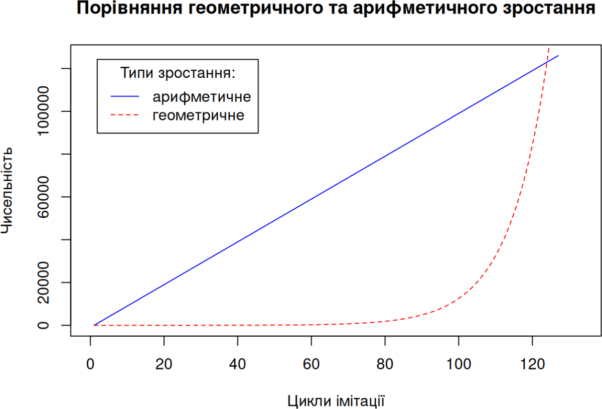
Comparison (and "race") of arithmetic and geometric growth.
# "ПЕРЕГОНИ" АРИФМЕТИЧНОГО ТА ГЕОМЕТРИЧНОГО ЗРОСТАННЯ
# INITIAL SCRIPT COMMANDS — ПОЧАТКОВІ КОМАНДИ СКРИПТУ:
N1 <- 1 # Початкова чисельність популяції (однакова для обох прогресій)
rm(list = ls()) # Очистка Environment
# E_N_T_R_A_N_C_E — В_Х_І_Д_Н_І___К_О_М_А_Н_Д_И
# MAIN PARAMETERS — ГОЛОВНІ ПАРАМЕТРИ:
N1 <- 1 # Початкова чисельність популяції (однакова для обох прогресій)
a <- 1000 # Доданок арифметичної прогресії. Показує, яка величина додається до кожного попереднього значення арифметичної прогресії
q <- 1.1 # Знаменник геометричної прогресії. Показує, на яку величину множиться кожне попереднє значення геометричної прогресії
# EXPERIMENTAL CONDITIONS — УМОВИ ЕКСПЕРИМЕНТУ:
cycles <- 1000 # Тривалість експерименту (максимальна кількість кроків))
# W_O_R_K_S_P_A_C_E — Р_О_Б_О_Ч_И_Й___П_Р_О_С_Т_І_Р
# GENERAL OBJECTS CREATION — СТВОРЕННЯ ГОЛОВНИХ ОБ'ЄКТІВ:
arithm <- rep(NA, cycles) # Створення пустого вектора для запису арифметичної прогресії
geom <- rep(NA, cycles) # Створення пустого вектора для запису геометричної прогресії
# INITIAL STATE OF THE SYSTEM — ПОЧАТКОВИЙ СТАН СИСТЕМИ:
arithm[1] <- N1 # Перенесення першого значення арифметичної прогресії
geom[1] <- N1 # Перенесення першого значення геометричної прогресії
# W_O_R_K_F_L_O_W — Р_О_Б_О_Ч_И_Й___П_Р_О_Ц_Е_С
for(t in 2:cycles) { # Цикл, що перебирає кроки імітації
  arithm[t] <- arithm[t-1] + a # Добудова обох прогресій
  geom[t] <- geom[t-1] * q
  if (t>5) if(geom[t-3] > arithm[t-3]) break # Перевірка, чи не перегнала геометрична прогресія аріфметичну (три кроки тому, щоб результат перемоги потрапив на діаграму)
              }
# F_I_N_I_S_H_I_N_G — З_А_В_Е_Р_Ш_Е_Н_Н_Я
# RESULTS VISUALIZATION — ВІЗУАЛІЗАЦІЯ РЕЗУЛЬТАТІВ:
plot(arithm,  xlim=c(0, t*1.05), type="l", lty=1, col="blue",
     main="Порівняння геометричного та арифметичного зростання",
     xlab="Цикли імітації", ylab="Чисельність")
lines(geom, type="l", , lty=2, col="red")
legend("topleft", inset=.05, title="Типи зростання:", c("арифметичне", "геометричне"), lty=c(1, 2), col=c("blue", "red"))