

SexOnR–12_Fisher. Modeling Fisher’s Equilibrium (Task III)
Why do we observe a sex ratio of 1:1 in many dioecious populations? Imagine a population in which only one tenth of the individuals are males (each of whom, on average, fertilizes nine females). Such a population would not “pay” the double cost of sex, because only one tenth of the resources would be spent on producing males! Why do we not observe such populations?
10 Modeling Fisher’s equilibrium
10.1 Problem statement
Why do we observe a 1:1 sex ratio in many dioecious populations? Imagine a population in which only one tenth of the individuals are males (each of whom, on average, fertilizes nine females). Such a population would not “pay” the double cost of sex, because only one tenth of the resources would be spent on producing males! Why do we not observe such populations?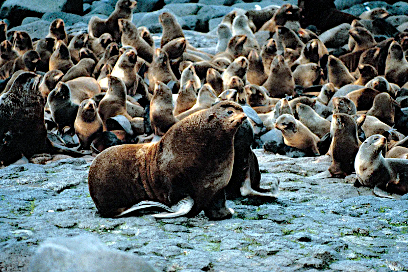
Fig. 10.1.1. A seal hareem. One male is accompanied by a large number of females. Is it worth producing more males than are needed to form harems?
The answer to this question is associated with Ronald Fisher’s name, although it is noted that he was not the first to understand the principle we will discuss and study here, and that Charles Darwin had already understood the idea.
To explain this answer, we can begin from afar. Population reproduction is a consequence of organismal reproduction. It may be that optimizing these processes at the population level and at the organismal level will differ. Among populations we observe some that prove more stable, including in competition with other populations (this was discussed in more detail in the lecture Evolution and Sex). Likewise, the traits of organisms are shaped by selection for the stability of their reproduction. Some traits are beneficial both for the survival of the individual and for the survival of the population. For example, in Fig. 10.1.1 we see animals with streamlined bodies, highly adapted to swimming and hunting fish. This promotes both individual survival and population stability. However, some traits may be beneficial for populations and harmful to organisms, or vice versa. Thus, we may suppose that it would be advantageous for a population if only 10% (or some other relatively small fraction) of the individuals produced were males. But would the trait of maintaining the production of mostly females be favored by selection at the organismal level?
To answer the last question, let us recall several important points:
- organisms are shaped by selection for the stability of their reproduction;
- the measure of how strongly a given organism should be favored by selection is fitness;
- fitness is calculated as the expected contribution to the next generations;
- in dioecious organisms, each individual has one mother and one father.
Suppose there is a population in which one tenth of the offspring are males - nine times fewer than females. In that case, each male would have nine times more offspring than each female! We know that there are cases in which certain parents produce mostly sons or mostly daughters. In such cases, any changes that increase the probability of male offspring will be favored by selection. As a result, the fraction of males will increase until it reaches one tenth. Can such selection lead to there being more males than females? No. If males became more common, selection would begin to favor females. This situation is an example of frequency-dependent selection, that is, selection that supports or rejects certain forms depending on how common those forms are in the population.
Fisher’s equilibrium is a problem that has received much attention. Among other things, the discussion and analytical modeling of this problem contributed to the development of game theory. Nevertheless, the problem remains interesting for modeling.
I invite students to build a simulation model of selection on the sex ratio in offspring. Once this model works in its “pure” form, it will be possible to use it to explore other interesting questions. How will the sex equilibrium shift if producing a male requires greater costs than producing a female (Fisher gave an answer to this question)? How will different life spans of females and males, or different probabilities of death for the two sexes, affect the sex ratio?
10.2 Designing the conceptual model “Fisher’s principle”
Let us begin designing the model (however, it should be remembered that during implementation it may become necessary to revise the original design).
We need to simulate a dioecious population with constant size. We will need the following initial parameters:
K — carrying capacity, the Verhulst parameter: the number of individuals beyond which population size is reduced;
r — fecundity, the Malthus parameter: the number of offspring per breeder per model cycle.
In the previous models (Maynard Smith and Sturtevant), the individuals were “immortal”: at each cycle, the number of offspring was simply added to the number of parents. This makes sense if all individuals of a given sex (or, say, a given mode of reproduction and genotype, if the number of genotypes is small) are identical. In this model we study selection on traits that affect the sex distribution of offspring. It probably makes sense to consider a sufficiently large number of genotypes (at least 10, perhaps more). In that case each individual in our model receives a certain individuality. Let us characterize this individuality by three traits: sex, age, and an innate tendency toward a particular sex distribution in offspring.
In general, the transformations that should occur during the model’s main working cycle will be as follows.
αtP, alpha composition: initial composition for each cycle
↓ pairing and reproduction, parents “age”
βtP, gamma composition: parents and offspring together, parents aged by one cycle
↓ selection (depending on sex and age, if needed)
γtP, delta composition: population after selection
↓ nonselective reduction
ωtP, omega composition: final composition at the end of the cycle
If individuals in the model differ by sex, age, and expected probabilistic sex distribution among offspring, these traits must be encoded somehow. Let us encode sex in tens of thousands (females — 10000+; males — 20000+), age in hundreds, and the expected probabilistic sex distribution of offspring in units (we will denote the fraction of female offspring produced by a given individual). In that case, code 10307 corresponds to a female three model cycles (“years”) old, who, when paired with a male coded 20307, produces 7 daughters and 3 sons.
An important question is how exactly to determine sex and the tendency toward sex distribution in offspring (age is simpler: the number of cycles equals the age). One possible option is to determine these by means of an array that enumerates all possible mating combinations.