StatOracle–01 Core Concepts of Biostatistics

1 Core Concepts of Biostatistics
1.1 What is biostatistics, and why is it needed
Statistical analysis of the results of biological research allows one to solve several types of problems:
— to present visually the results describing the diversity of the objects under study;
— to accept or reject, with justification (at a given probability of error), assumptions about the existence of regularities reflected in the variability of the quantity under study;
— to reveal implicit regularities hidden within the variation of the data being studied.
One should not assume that there exists some special biological statistics that is fundamentally different from mathematical statistics in general. Nevertheless, the variability of biological objects has certain features that distinguish them from, for example, the variability of financial indicators or the results of industrial technological processes. This leads to the set of methods used in biology differing from those used in other fields of statistical application. In addition, it should be remembered that statistical analysis in biology is not an end in itself: it is subordinate to the objectives of biological research and cannot be fully interpreted outside the scope of the biological problem under investigation. Furthermore, not only must data analysis be subordinate to the logic of biological research, but the research itself must be designed with future analysis in mind. The collection of empirical data and the design of experiments must account in advance for how the resulting data will be analyzed. Thus, although the application of statistics in biology cannot be entirely separated from mathematical statistics per se, or from the fields of biology studied by means of statistical methods, it nonetheless constitutes a distinct scientific domain associated with a particular complex of problems and methods for their solution. For this domain one may use the term proposed in 1899 by Francis Galton — biometry. However, since the term “biometry” has been appropriated by specialists in personal identification by individual characteristics, in many contexts it is simpler to use the term biostatistics.
The objects studied by biology have a high degree of uniqueness. In virtually any biological phenomenon, both general regularities and the influence of particular circumstances are manifested, often related to one or another uniqueness of biosystems. This means that methods enabling the detection of general regularities manifested in the variability of individual observations are of great importance for biological research. Perhaps this is why biologists have made a substantial contribution to the development of statistics as a whole. The results of the work of Francis Galton, Karl Pearson, Ronald Fisher, and other outstanding biologists constitute an important part not only of biostatistics but of mathematical statistics in general.

1.2 Probability
Only repeatable events can be studied statistically. For example, we select rabbits blindly from a box. The rabbits may be black or white. Each selection is an elementary event. A person inserts their hand into the opening of the box, blindly feels for a rabbit, and grasps it… Can one know in advance which rabbit the person will draw? No (if there are no other sources of information and no other factors influencing the outcome). If we know that the box may contain both white and black rabbits, we cannot be certain of the color of the animal that will be drawn.
As soon as the rabbit is pulled out, we do more than simply learn its color. If we did not previously know which rabbits were in the box, we have obtained certain information about the composition of the population from which a given representative was selected. For example, if a white rabbit was drawn, we can assert that there was at least one white rabbit in the box. Not much… But if ten rabbits are drawn in succession, the composition of the group gathering at the feet of the person drawing them will allow a more justified assumption to be made about the composition of the rabbits in the box. These assumptions are grounded in the phenomenon of probability, which manifests itself in regular, repeatable events. Probability is a numerical measure of the possibility of an event. A probability of 1 means that the event will certainly occur, while a probability of 0 means that it is impossible.
Suppose we know that the box contains 50 white and 50 black rabbits. What is the probability of randomly selecting a white rabbit in a single draw? Of the total number of possible outcomes (100), 50 satisfy this condition, so the probability is 50/100 = 1/2 = 0.5. How probable is it to select two white rabbits? These are independent draws, so their probabilities must be multiplied (Fig. 1.2.1). It might seem that the probability of obtaining two white rabbits equals 0.25, although in reality it is somewhat less. After a rabbit of a given color has been selected, the probability of selecting a second of the same color is 49/99 versus 50/99. Therefore, the probability of selecting two white rabbits is 0.24747…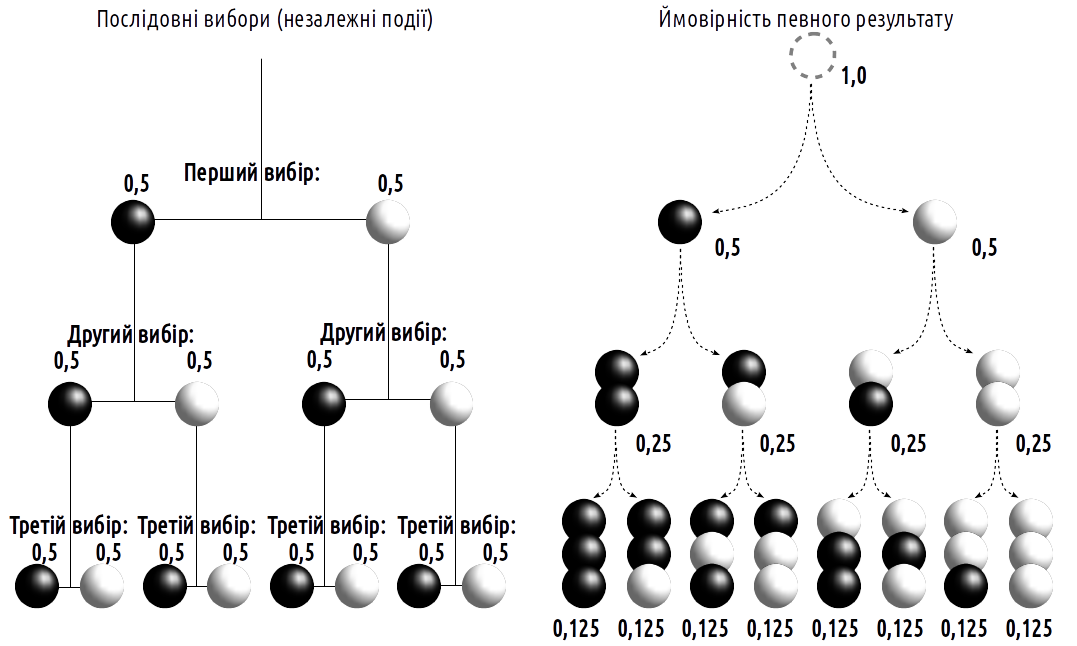

Fig. 1.2.1. When calculating the probability of a combination of independent events, their probabilities are multiplied
Should one consider the possibility that, for example, the hand withdrawn from the box holds no rabbit at all, or perhaps two at once? In real life — yes; in the simplified model to which the apparatus of elementary probability theory can be applied — one need not account for this. Those cases in which a person retrieves no rabbit, or retrieves two at once, do not conform to the conditions of a single draw. However, were the reader of this text to insert their hand into a real box filled with rabbits that kick and struggle as best they can, the probability of retrieving nothing could not be neglected.
1.3 Population and sample
A population (general population) is the actual or hypothetical totality of all objects belonging to the category under study. In most cases it is impossible to study the entire population, and researchers work with samples (empirical sets, sample sets) — groups of objects obtained from the population.
The size of the population is determined by the research objective (and may vary substantially depending on how the objective is formulated). Comparing the height of male and female students in a group studying biostatistics may constitute a study of that group itself (in which case the sample will encompass the entire population), a study of students at a particular university (where the population, though large, is at least finite), or a study of students or people in general (in the latter two cases the population, at least hypothetically, becomes potentially infinite).
A fundamental paradox of statistics is that a researcher works with samples while studying the populations from which those samples are drawn.
Can a sample serve as a basis for inference about a population substantially broader than the sample itself? To some extent, yes. It is clear, however, that not every sample reflects the composition of the population from which it was obtained. Can one draw a sample to study the diversity of human height from among university students? No, because such a sample would consist predominantly of young people who wished to pursue higher education and were able to gain admission to the relevant institution. Such a sample is biased. To obtain a fully random sample, the sampling process would need to be organized such that any object within the population had an equal probability of inclusion. In most cases such selection is practically impossible. Nevertheless, for the purpose of studying a population only representative (illustrative) samples should be used — samples in which deviations from random selection cannot lead to substantial bias. Even so, some representativeness error (deviation of the sample’s characteristics from those of the population) is inevitable whenever the population is broader than the sample under study.
The non-random character of the samples with which a biologist works is one of the constant (and entirely unavoidable) problems in biological research. Imagine that rather than drawing black and white rabbits from a box, we need to determine their ratio in a given habitat. How might this be done? For example, by going into the field and counting rabbits of each color encountered along the researcher’s route. However, on dark ploughed soil white rabbits will be more conspicuous, whereas after snowfall black ones will be. Perhaps instead of relying on the researcher’s eyesight, rabbits should be caught in traps? But if white rabbits are albinos, they may have poorer vision than black rabbits and fall into traps more often. A sample of rabbits observed during a transect survey and a sample of rabbits caught in traps are not fully representative for estimating the population of rabbits inhabiting the study area.
Now imagine that a zoologist is attempting to assess the composition of a sand lizard population. He visited the habitat of this population on a cloudy, windy day preceded by several consecutive days of rain. In such weather only young individuals and gravid (egg-bearing) females — those experiencing particularly intense hunger — came to the surface in search of food. The researcher collected several individuals that appeared to him to be “typical,” along with a few additional specimens that attracted his attention by their unusual appearance. In subsequent analysis he will draw inferences about the properties of the population under study (the given population) on the basis of the properties of the available sample. Unfortunately, no statistical analysis method can fully correct the bias of such a sample.

Examples of incorrect use of the words “reliability” and “significance” are frequently encountered. The concept of “statistical significance” (or simply “significance”) has a precise mathematical interpretation. The statistical significance of a given result (for example, the detection of a difference between groups of data or of a relationship between two variables) — is the low probability of its random occurrence. The statement “two samples differ statistically significantly” means that the probability of their having been obtained from a single population is so low that their having been obtained from different populations may be considered established. “Reliability” is a much broader concept that may be employed in the most diverse fields (from jurisprudence to philosophy) and has no mathematical definition. It is used to denote well-grounded, evidence-based knowledge. An example of correct application of such concepts is shown in Fig. 1.5.1.			Example
Incidentally, with poorly designed experiments or errors in interpretation, unjustified conclusions may appeal to a multitude of statistically significant phenomena; significant differences between samples of unreliable facts are of no significance whatsoever…	In the overwhelming majority of sources the practice is simply to speak of “significance levels.” This is by no means an error, and such usage is entirely permissible. However, on the grounds that this text is educational in character, the author will endeavor in all cases to use the full formulation: “statistical significance.”	1.6 Traits	When describing objects of study, researchers record the states of one or another trait — characteristics by which the objects being compared may differ from one another. Traits may be of different kinds.
	Table 1.6.1. Categories of traits	Categories of traits	Expressed as
	Example	Quantitative	Metric (continuous, measured)
(= dichotomous) (attributive)	Body length of a frog	Meristic (discrete, count)	An integer
	Number of stripes on the shank	Rank (ordinal)	An integer (rank), where the difference between ranks is not a measure of the difference between compared objects

Consider a humorous example. Everyone knows the trick in which a magician pulls a rabbit from a hat (Fig. 1.4.1). Where does the magician’s rabbit come from? Unknown… One might imagine that the hat is an entrance to something analogous to the box of rabbits we used to discuss the concept of probability. The procedure of obtaining rabbits from the hat can be compared to drawing a sample from a population. The sample consists of the rabbits drawn (perhaps one, perhaps more, one after another), while the population is the rabbits in that “magical,” hidden space from which they are extracted.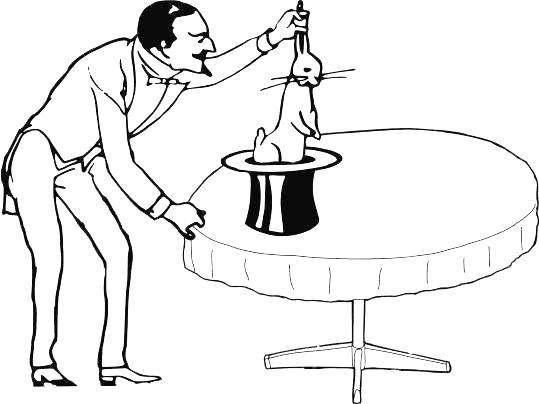

Fig. 1.4.1. What can we assert about the space from which the magician drew a rabbit (i.e., what can we learn in this case about the population from the sample we have obtained)?
There was at least one white rabbit there…
Suppose the magician draws rabbits blindly from two hats: whatever his hand grasps when inserted into a hat, that is what he draws. Inserting his hand into the first hat, he drew a white rabbit; inserting it into the second — a black one (Fig. 1.4.2).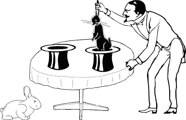

Fig. 1.4.2. From the second hat appeared a different rabbit, a black one… Do the two hats lead to the same space or to different ones (in other words, are the two samples drawn from the same population or from different ones)? We have insufficient grounds for choosing either alternative. The two samples may have been drawn from a single population containing both black and white rabbits, or from different populations.
Can we, from the composition of the rabbits in two samples corresponding to the two hats, determine whether they were obtained from a single population? Sometimes the data at hand cannot help us choose between mutually exclusive possibilities, and sometimes they can provide grounds for justified assumptions (Fig. 1.4.3).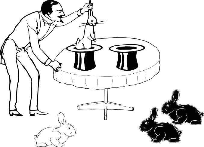

Fig. 1.4.3. More information for making a decision is now available… If we accept that through the two hats the magician reaches two different populations, no additional assumptions are needed. If both samples are drawn from a single population, we must assume that a relatively improbable outcome has been realized.
What is the probability that the magician will obtain two white rabbits in one sample and two black ones in the other, if he draws them from a single population? What ratio of white to black rabbits can we expect in the population (if it is one)? We know for certain that it contains both white and black rabbits, and their ratio can be estimated from the combined sample (in this case we assume that the differences between the rabbits from the two hats result from chance alone). The most probable scenario is equal numbers of white and black rabbits, since this is consistent with the overall sample obtained.
On the magician’s first draw into one of the hats, he retrieved a rabbit of some color. The scenario shown in Fig. 1.4.3 is realized when the rabbit drawn from that hat is of the same color (i.e., an event with probability we estimated at ½ occurs), and from the other hat two rabbits of the opposite color are drawn in succession (i.e., two further independent events each with probability ½). Thus, a distribution as shown in the figure would arise from a shared rabbit space in only one out of every eight attempts. It is more probable to suppose that the rabbit populations are different, although of course we have insufficient grounds to reject the assumption that the rabbits come from a single shared population…
Moreover, more complex cases are possible (Fig. 1.4.4)…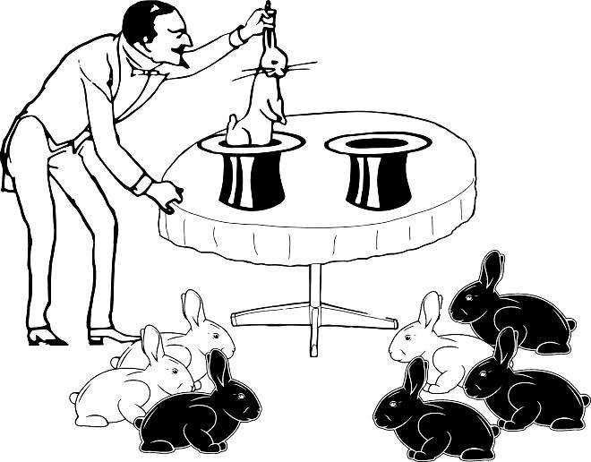

Fig. 1.4.4. Even more information is available, but the probability calculation is not as straightforward as in the previous case.
The overall ratio of white to black rabbits is the same as in the previous case. The probability that in one sample the ratio turns out to be 1 to 3 and in the other 3 to 1 (without taking into account the order in which the rabbits were drawn in each sample) proves to be the same as in the previous example: the result shown in Fig. 1.4.4 is observed in one case out of eight.
How will our assessments change if the samples become larger and the differences between them more pronounced (Fig. 1.4.5)?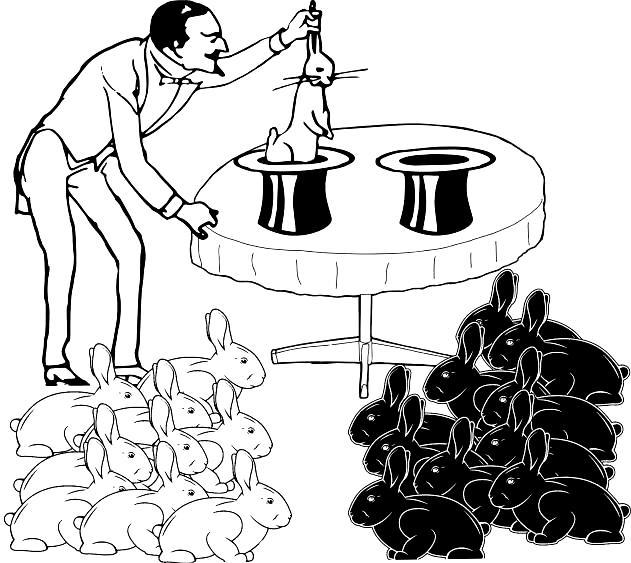

Fig. 1.4.5. In this case a fairly probable answer can be given to the question of whether the magician inserts his hands through different hats into the same space or into different ones: into different ones. If the space were one, a distribution of 10 rabbits of one color in one sample and 10 rabbits of the other color in the other sample could be observed only in one case out of 524,288 attempts.
If the rabbit samples obtained from two hats differ strongly (from one hat — 10 white, from the other — 10 black), the magician is almost certainly drawing rabbits from different spaces, from different populations. The probability that such a result is a consequence of chance is one divided by 2¹⁹. If we reject the assumption of such an improbable event, we will almost certainly not err. Thus, one may conclude that in the case shown in Fig. 1.4.5, the hats lead to different spaces. However, it is important to remember: we have not proven that the spaces to which the hats lead are different, but merely obtained grounds to assume their difference with high probability.
One might suppose that if the samples do not differ in composition (Fig. 1.4.6), we would have grounds for the opposite conclusion. Unfortunately, this is not so. If on the basis of sample composition we conclude that both hats are portals to the same place, we make an error. We have established only that the assumption of equal ratios of white to black rabbits in the populations to which the two hats in Fig. 1.4.6 lead is consistent with the composition of the rabbits drawn from them. But we have no grounds for choosing between the assumption that these are two different spaces with identical composition, and the assumption that they constitute a single shared space.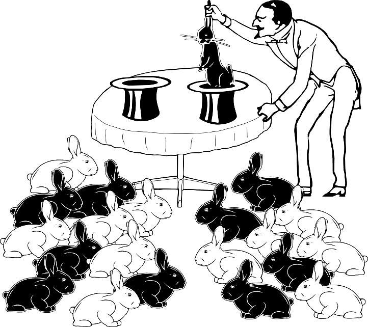

Fig. 1.4.6. Is this distribution of rabbits consistent with the assumption that through the two hats the magician inserts his hands into different spaces? Perfectly consistent!
Thus, the case in Fig. 1.4.5 provides grounds for a definite conclusion, whereas the case in Fig. 1.4.6 does not. This reflects a general principle: by comparing two samples, we can sometimes prove that they come from different populations (i.e., justify that the opposite conclusion is extremely improbable), but we cannot prove that they come from the same population. Nevertheless, one can justify that the difference between the populations from which the samples were obtained does not, with a given probability, exceed a certain level…
In the case of comparing samples as considered in this example, the probability that the samples were obtained from one population and that the differences between them are a consequence of chance is called the statistical significance of the assumption that the populations from which the samples were drawn are different. In other cases (for example, when studying the relationship between the variability of two traits), statistical significance is defined analogously — it is the probability that the observed effect is a consequence of chance. Briefly: the significance level is the probability that the observed result is a consequence of chance in the formation of the samples.
What does the phrase “the result is statistically significant” mean? It means that the random occurrence of this result is very improbable, that we have every reason to regard the result as non-random and as reflecting genuine features of the object of our study.

1.7 Distributions, statistics, and parameters	A distribution is a function describing the probability of various values of a randomly varying quantity. The fact that a coin may fall heads or tails with equal probability defines the distribution of coin-toss outcomes.
Random variables (and their distributions) may be discrete or continuous. Quantitative and count traits have discrete distributions; metric traits have continuous distributions. n.
Samples can be described by assuming that the distribution of values within them follows some law characteristic of the population from which the sample was drawn. ,	Suppose the sample under study consists of the results of some measurements. For the sample, its mean value can be computed. If the sample is fully described, its mean can be determined exactly. On the basis of the sample mean, one can judge, with a certain degree of precision, the mean value of the population from which the sample was drawn.
Mathematical quantities characterizing a sample are called statistics and are denoted by Roman (Latin) letters; quantities characterizing the population are called parameters and are denoted by Greek letters. s;	In the typical case, in the course of a biostatistical study the parameters of the population are inferred from the statistics of the sample.

To formalize such reasoning as we engaged in in the previous section, it is customary to formulate two hypotheses between which a choice must be made in the course of a statistical study.
The null hypothesis (H₀) asserts that there are no differences between the populations from which the samples were drawn (and that the difference between the samples is a consequence of chance in their formation).
The alternative hypothesis (H₁) asserts that the differences between the samples reflect differences between the populations from which those samples were drawn.
A definitive choice between these possibilities cannot be made, and the possibility of error always remains. On the basis of the available sample composition data, one must estimate the probability of the null and alternative hypotheses and make the optimal decision. For this choice, statistical tests are used — rules enabling such a choice to be made.
Both the null and alternative hypotheses may be non-directional (where the researcher is interested in the mere fact of a difference between the populations from which the samples were drawn) or directional (where it matters specifically how the samples differ; for example, it is asserted that a given influence increases the value of the trait under study; in the population subjected to the influence, trait values are higher). For example, when determining whether sex affects tail length, we may treat both the case in which the tail is longer in females than in males, and the case in which it is shorter, as confirmation of such an effect. When determining whether a new treatment “works,” confirmation of the alternative hypothesis will consist only of the case in which the method under study promotes recovery. The alternative hypothesis must specifically be that the treatment promotes recovery. Consequently, in the first case non-directional tests should be applied, and in the second — directional ones. The level of statistical significance can be defined as the probability of making an error. From this perspective, the level of statistical significance is the probability that we will treat an effect as significant (choose the alternative hypothesis) when it is in fact a random one. Such an error — accepting the alternative hypothesis when it is false — is called a Type I statistical error. A Type II error is the acceptance of the null hypothesis when the alternative is correct. As a rule, Type I errors prove more dangerous. The probability of a Type I error is denoted α, and of a Type II error — β.
In simpler terms (without reference to two hypotheses), significance can be defined as follows. Statistical significance is the probability that the result obtained in the course of a study is explained by chance in the formation of the sample.
Examples of incorrect use of the words “reliability” and “significance” are frequently encountered. The concept of “statistical significance” (or simply “significance”) has a precise mathematical interpretation. The statistical significance of a given result (for example, the detection of a difference between groups of data or of a relationship between two variables) — is the low probability of its random occurrence. The statement “two samples differ statistically significantly” means that the probability of their having been obtained from a single population is so low that their having been obtained from different populations may be considered established. “Reliability” is a much broader concept that may be employed in the most diverse fields (from jurisprudence to philosophy) and has no mathematical definition. It is used to denote well-grounded, evidence-based knowledge. An example of correct application of such concepts is shown in Fig. 1.5.1.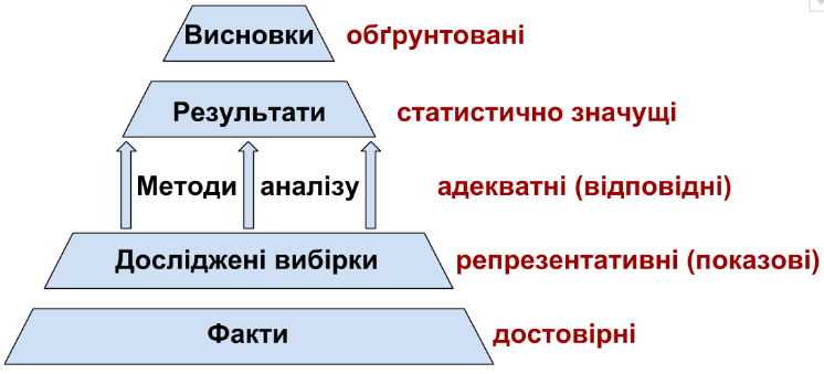

Fig. 1.5.1. Application of concepts describing correctly conducted work.
Incidentally, with poorly designed experiments or errors in interpretation, unjustified conclusions may appeal to a multitude of statistically significant phenomena; significant differences between samples of unreliable facts are of no significance whatsoever…
In the overwhelming majority of sources the practice is simply to speak of “significance levels.” This is by no means an error, and such usage is entirely permissible. However, on the grounds that this text is educational in character, the author will endeavor in all cases to use the full formulation: “statistical significance.”
1.6 Traits
When describing objects of study, researchers record the states of one or another trait — characteristics by which the objects being compared may differ from one another. Traits may be of different kinds.
Table 1.6.1. Categories of traits

Traits from different groups differ in their properties. For example, an individual with four stripes on the shank differs by the same number of stripes from an individual with three, as an individual with three stripes differs from one with two. In contrast, with respect to individuals differing in the rank of the first digit’s length on the forelimbs, it is impossible to state by how much the digit in an individual with rank 4 is shorter than in an individual with rank 3, and the difference between individuals of rank 4 and 3 cannot be compared with the difference between individuals of rank 3 and 2.
Thus, traits are characteristics by which objects can be compared with one another. The result of describing an individual in terms of a given trait is called the state or value of that trait. When working with a computer program, what is entered into an individual cell of a data table is most simply referred to by the term “value” (though other variants exist, for example “data point”).
1.7 Distributions, statistics, and parameters
A distribution is a function describing the probability of various values of a randomly varying quantity. The fact that a coin may fall heads or tails with equal probability defines the distribution of coin-toss outcomes.
Random variables (and their distributions) may be discrete or continuous. Quantitative and count traits have discrete distributions; metric traits have continuous distributions.
Samples can be described by assuming that the distribution of values within them follows some law characteristic of the population from which the sample was drawn.
Suppose the sample under study consists of the results of some measurements. For the sample, its mean value can be computed. If the sample is fully described, its mean can be determined exactly. On the basis of the sample mean, one can judge, with a certain degree of precision, the mean value of the population from which the sample was drawn.
Mathematical quantities characterizing a sample are called statistics and are denoted by Roman (Latin) letters; quantities characterizing the population are called parameters and are denoted by Greek letters.
In the typical case, in the course of a biostatistical study the parameters of the population are inferred from the statistics of the sample.
Table 1.7.1. The most common statistics and their corresponding population parameters

Sample size — n.

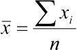
Arithmetic mean — ,

Population mean —

Standard deviation — s;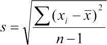

Population standard deviation —

Arithmetic mean (Mean) , where is the arithmetic mean of the variable x under study; n is the number of elements in the sample; xᵢ are the individual values of the variable x, from x₁ to xₙ. Individual values obtained from different samples can be regarded as sample estimates of the population mean (the arithmetic mean of the population encompassing the entire set of objects represented by the sample under study).
Variance, mean-square deviation (Variance). The population standard deviation could be computed as , but to do so it would be necessary to enumerate all elements of the population. In practice, this parameter is always determined for a given sample, which in all likelihood will not include the rarest elements that deviate most strongly from the mean. Accordingly, the sample variance, denoted s², must be computed with a correction. For this purpose the formula is used. The quantity df = n−1 has been named the number of degrees of freedom. It may be considered that, given a known , all elements of the sample except the last can be freely varied (i.e., their number equals n−1): once all other values and the mean are determined, the last value in the sample is uniquely determined by these quantities.
In Ukrainian and Russian, variance is often called dispersiya (from Latin dispersio — scattering, which also gives rise to the name of analysis of variance). It is sometimes noted that the term dispersiya should be applied only to denote the very fact of the scattering of individual values around the mean, while the described measure should be called, by analogy with English, variance. Variance is the square of the standard deviation, which is denoted s and computed as .
Other statistics characterizing samples are also sometimes used. These include the range (the difference between the minimum and maximum values), the median (the value located exactly in the middle of the ordered sequence of sample elements, such that half the elements are smaller than this value and half are larger), the mode (the most numerous class of values in the sample), the mean absolute deviation, the geometric mean, and so forth. A sound analysis of these and other statistics can be found here.
In accordance with the law of large numbers, the history of which goes back to J. Bernoulli (1713) and which was proven by P.L. Chebyshev in the nineteenth century, as the sample size increases, the sample statistics tend toward the parameters of the population. The smaller the sample, the more likely the deviation of sample statistics from the population parameters.
If a metric trait is influenced by many random factors, it acquires a normal distribution. Graphically, this distribution is described by the normal curve, which is uniquely determined by just two parameters: and .
In the normal distribution, the mean, median, and mode coincide. Under a normal distribution, 99.7% of observed values lie within (the three-sigma rule).
Empirical distributions may resemble normal distributions but differ from them. The most common measures for assessing such differences are skewness and kurtosis.

1.8 Parametric and non-parametric statistical methods and tests
Statistical tests (rules enabling a choice to be made between the null and alternative hypothesis) can be divided into parametric (those whose computational procedure assumes that the samples being compared were drawn from populations with a particular — most often normal — distribution) and non-parametric, or distribution-free (their computations require no assumptions regarding the nature of the distribution of the populations under study). Accordingly, if we do not know how the quantities we are studying are distributed, we should by default use non-parametric methods. However, most non-parametric methods are less powerful. Since the probability of committing a Type II statistical error (i.e., “missing” a difference, accepting the null hypothesis when the alternative is true) is denoted β (Section 1.5), the power of a statistical test can be defined as 1 – β. This is entirely logical, since parametric methods already “know” something about the distributions of the quantities being compared.