Creation of Worlds — 04. Incorporating Demographic Structure: "The Three-Generation Model"

4. Incorporating Demographic Structure: "The Three-Generation Model"
4.1. New Capabilities
The models describing exponential and logistic growth that we considered at the previous stages of our course remain extremely schematic and detached from reality. In effect, we adapted analytical relationships to step-by-step computation using difference equations (equations that compute the difference between the value of a given quantity at the previous and the next step). We did not exploit in full the key advantage of simulation models — the ability to sequentially model various processes occurring in the original system at each cycle of its dynamics. Let us attempt to remedy this omission.
To begin with, let us construct the simplest possible model. We will introduce two sexes, three generations, and mortality resulting from competition when population size exceeds carrying capacity (this is not logistic growth, but rather exponential growth that is "trimmed" each time carrying capacity is exceeded by the modeled population). This model should not be regarded as definitive, but its construction will allow us to examine certain important principles of simulation model design. We will build this model so as to illustrate a particular template for arranging a model on a LO Calc worksheet. We will designate this template conditionally as the "Table with Header." Starting from this model, we will adhere to the notation style that may be called "recommended" (in this course), at least for population-ecological models. The list of notations used in such models is given here. In addition, in constructing this model we employ two features we have not yet applied: the use of named cells and scroll bars for controlling input parameters.
We begin by examining the appearance of the model implementation (Fig. 4.1), and then discuss its construction.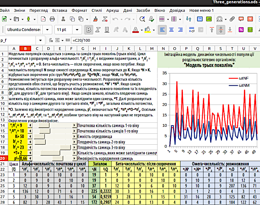

Fig. 4.1. General view of the implementation of the "Three-Generation Model"
In Fig. 4.1 we see the following elements: the title (N1:V3); an information field with a model description (A1:M13); a control zone for initial parameters (A14:M20); a zone for displaying simulation results (N4:V20); and a calculation zone (A21:V...?). As you will have understood, the position of each zone is indicated in the manner used in spreadsheets to denote rectangular regions: by the coordinates of the upper-left and lower-right corners.
The model description employs the "recommended" notation style, which takes the following form: stagecycleindicatorformage. Let us explain what is meant by these concepts:
— indicator: the notation proper for the quantity in question; for example, the size of a group is denoted n, while the total size of a given set of groups is denoted N;
— stage: a part of the cycle; each cycle is subdivided into the required number of transformation stages, denoted by Greek letters (as left superscripts); according to this logic, a cycle can be represented as a set of transformations αtN → βtN → γtN → δtN → εtN → … → ωtN;
— cycle: the sequence of transformations repeated in the course of model operation, which may, for example, correspond to the annual cycle in the life of a given population; denoted by a number as a left subscript, and in generalized form (as in the example with stage notation) — by the letter t;
— form: genotypes, sexes, or other categories of individuals; denoted by a right superscript, e.g., in the model under discussion — F (females) or M (males); in generalized form, the notation g (genotypes) may be used;
— age: individuals of a given form may be of different ages; a group consists of individuals of the same form and the same age; age is denoted by a digit as a right subscript; in generalized form, the notation a (age) is used.
This notation form may be written concisely as: α→ωtZga. Here α→ω denotes the Greek letters indicating stages, t is the cycle number of simulation and computation, Z is the indicator under consideration, g is the genotype, sex, form, or other category of individuals, and a is age.
You will have understood why in Fig. 4.1, in the column headings, the letter F in the notation for the number of sexually mature females ωtNF is uppercase, while in the notation for the number of pairs involving second-age females ωtPf2 the letter f is lowercase. This is admittedly not the most fundamental point, but it helps to understand the peculiarities of the notation style. When referring to the number of females, individuals of two groups are implied: second-year females and third-year females. When referring to the number of pairs including second-year females, they belong to one and only one group. In the first case the letter F denotes a category encompassing more than one group; in the second case the letter f denotes a single group.
You will now be able to understand the model description, which reads as follows:
The model population consists of females and males of three generations (three ages). The cycle begins with the computation of alpha-abundance. α1nf1 and α1nm1 are input parameters, while α1nf2 = α1nf3 = α1nm2 = α1nm3 = 0. Beta-abundance is computed after reduction, if reduction is required. If population size N exceeds carrying capacity K, it is reduced to K. If αN > K, all groups are reduced: βnga = αnga × βQ, where βQ = αN/K; if αN ≤ K, then βnga = αnfa. Reproduction is simulated when computing omega-abundance. The numbers of individuals of both sexes, ωNF and ωNM, are calculated. If males are sufficiently numerous, offspring number is determined by the number of females of each generation and their fecundity (bf2 for the second age and bf3 for the third age). If males are scarce, the number of fertile females depends on the number of females that one male can fertilize, ωT. Next, the number of pairs with second-age and third-age females, ωPF2 and ωPF3, is calculated, followed by the total number of offspring, ωO. Depending on the probability of female birth, pf, ωnf0 is determined; ωnm0 = ωO − ωnf0. Since αt+1ng1 = ωtng0, αt+1ng2 = βtng1, and αt+1ng3 = βtng2, third-age individuals do not carry over to the next cycle. All rounding is probabilistic.
We begin constructing the model by considering the use of named cells. In truth, the model under discussion is sufficiently uncomplicated that one could easily dispense with individual names for the input parameters. However, using this model as an example, we must learn the template that may be applied to more complex models as well. If you build a sufficiently complex model, one of the problems you will encounter in working with it is the writing — and, more importantly, the verification — of formulas. Quite often these formulas occupy several lines... How does one make sense of them? By using individual names for input parameters! This will substantially improve the readability of formulas.
As you can see in Fig. 4.1, the model explicitly specifies 7 input parameters (in fact, there are 4 more parameters — the initial sizes of second-year and third-year cohorts — but we set these to zero by default). Each of the 7 cells containing initial parameters has been assigned its own name. To assign a name to a cell, select it and then follow the path "Sheet / Named Ranges and Expressions / Define...". Certain character combinations cannot be used as names (for example, a name cannot coincide with the designation of any other cell, i.e., it cannot be a combination of a letter and a number). A cell may be named with a single letter, but not any letter; the name U will be accepted, whereas the name T will not. Underscores (_) may be used in names.
To view and edit the complete set of names, a separate dialog window may be opened. It opens via "Sheet / Named Ranges and Expressions / Manage Names...", or by expanding the menu located next to the cell address field in the upper-left corner of the LO Calc worksheet. If you select "Manage Names...", you enter a dialog where you can define, modify, and delete individual cell names (Fig. 4.2).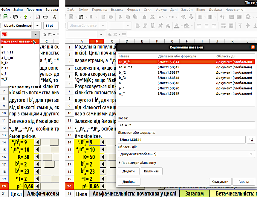

Fig. 4.2. Naming cells. On the left is shown where the "Manage Names..." dialog must be called. On the right is that dialog for the model we are about to construct.
Now, to insert into a formula a reference to cell B16, it suffices to simply write K. This reference is absolute and does not change when cells are stretched, copied, or moved.
When working with a model it is very useful for the input parameters to be displayed as clearly as possible and for their modification to be as convenient as possible. This can be facilitated by the use of scroll bars. These are one type of control element provided by spreadsheet applications. The simplest way to insert a scroll bar into a file is to copy it from a file in which one already exists. The more complex (but more correct) way is as follows. Follow the path "View / Toolbars" and select the "Form Controls" toolbar. This toolbar will appear on the LO Calc worksheet. Enter design mode using the "Design Mode" button (Fig. 4.2). Control elements will become accessible, among which you may select the scroll bar (Fig. 4.3). Having selected it, outline some area on the worksheet; LO Calc will insert the control element there. Depending on the area you outline for this element, it will be either horizontal or vertical.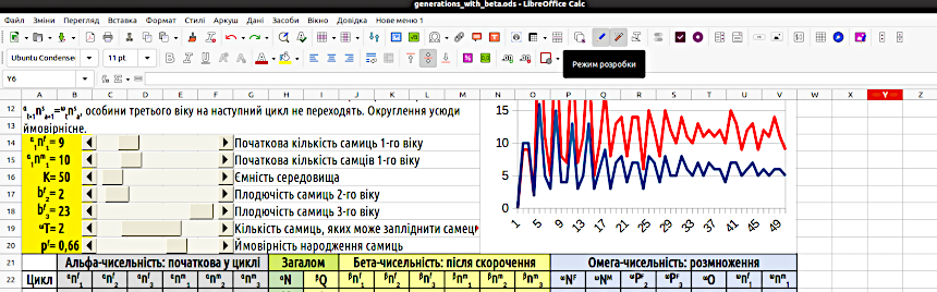

Fig. 4.3. This figure shows a fragment of the customized LO Calc toolbar, which also includes the "Form Controls" panel. In different versions of LO Calc the "Design Mode" button may have a different appearance. In any case, it is important to keep track of whether the button is pressed or not.
When design mode is enabled, you may place control elements on the worksheet and modify their properties. In this mode, however, the elements do not function. After setting everything up as required, you should exit design mode; the control elements will then "come to life." Select the scroll bar (Fig. 4.4).

Fig. 4.4. Now the scroll bar can be selected, placed on the LO Calc worksheet, and configured.
If the toolbar is active but the "Scroll Bar" button is absent from it, follow the path "Tools / Customize..." and configure which menus and buttons you wish to see on your screen (Fig. 4.5).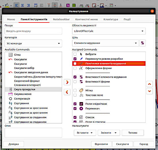

Fig. 4.5. Configuring toolbars.
To place a scroll bar on the worksheet, select this control element from the toolbar and "drag" the cursor to define the zone where it is to be located. This can only be done in design mode. After you have placed the bar, the "Control Properties" button becomes active (in addition, this mode may be selected via the right-click context menu). You will enter the "Properties: Scroll Bar" dialog. This dialog opens on the second tab, "Data"; there you must specify the cell whose value will be changed by means of this scroll bar (Fig. 4.6).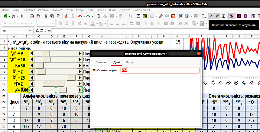

Fig. 4.6. Configuring the last scroll bar (highlighted by green markers). Note: the bar controls a cell in column C; the cell in column B that sets the input parameter depends on this cell.
On the first tab, "General," you can configure the scroll bar properties, which include dimensions, position, the minimum and maximum values that can be set with this scroll bar, the step increment, its orientation and size, and so forth (Fig. 4.7). If you think that fitting scroll bars and similar actions are superfluous embellishments, you are mistaken. Attention to detail makes it possible to create models that are easy to interpret and relatively free of errors.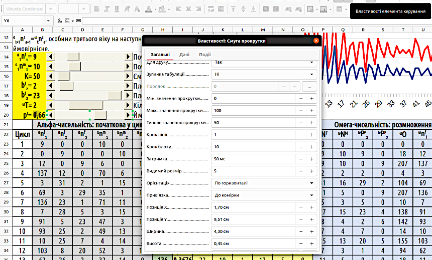

Fig. 4.7. In this dialog, all scroll bar properties can be flexibly configured. Incidentally, how do you think the author achieved such neat alignment of the scroll bars as shown in this screenshot?
After the control element's properties have been configured, the dialog window may simply be closed: the changes will be saved. Note that the scroll bar will only become functional once you exit design mode! To change the position of the bar or its other properties, you will need to enter design mode again.
As you will have understood, in the model you are about to create, the cells containing initial parameters must be named and linked to scroll bars, so that the values of these parameters may be changed as conveniently as possible. In the screenshot you can see 7 scroll bars; 6 of them alter cells in column B, while the last one alters a cell in column C (Fig. 4.6). The reason is as follows: scroll bars cannot be used to set non-integer values. The last bar changes the value of the cell in the range from 0 to 100. As you can see in Fig. 4.1 (note the cell address and the formula it contains!), cell B20 is calculated on the basis of the value in cell C20. Cell C20 itself is concealed beneath the scroll bar so as not to interfere with the model user.
4.2. Computations in the "Three-Generation Model"
In the preceding section we described the implementation features of the "Three-Generation Model." Here we must discuss how the conceptual model — whose implementation we have examined — is constructed. We must consider what relationships connect the quantities we examine in this model.
We vary 7 input parameters, to which (Fig. 4.2) names have been assigned (from top to bottom): a1_n_f1, a1_n_m1, K, b_f2, b_f3, w_T, and p_f.
Visualization of the output data is presented as an ordinary graph, which you already know how to construct, while we shall now analyze in detail the structure of the calculation field. As you can see in the screenshots, computations begin from row 23. To illustrate the discussion, we shall examine screenshots of the model in which the cell values are replaced by the formulas they contain (Fig. 4.8 and Fig. 4.9). To enter this mode, issue the command "View / Show Formula."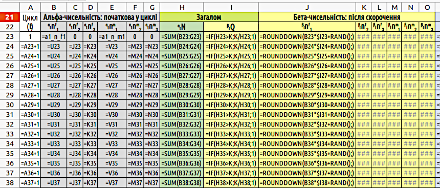

Fig. 4.8. Formulas in the first part of the "Three-Generation Model." Beta-abundance computations are of the same type and are shown only for the first column.
Column A contains the cycles of model operation (which in practice may correspond, for example, to years). The first row in the calculation zone is the zeroth cycle, A23{1}. The second cell in this column, A24, like all subsequent cells ("stretched" from A24), contains the simplest counter: A24{=A23+1}.
Column B specifies the number of first-year females at the beginning of the cycle — αtnf1. The formulas in the cells are: B23{=a1_n_f1}, B24{=U23}; all subsequent cells in this column are obtained by "stretching" from B24. The meaning of this difference is straightforward. Cell U23 contains the number of females in the offspring that could have appeared at the previous model step. That there is no offspring at the first cycle is of little importance; had there been individuals capable of reproduction in the first cycle, offspring would have appeared as well. We enter into these cells formulas that can be "stretched" across the entire model.
Column C specifies the number of second-age females at the beginning of the cycle — αtnf2. The formulas in the cells are: C23{0} (by the initial conditions, all individuals at the beginning of model operation belong to the first age class), C24{=J23}; all subsequent cells in the column are obtained by "stretching" from C24. Cell J23 specifies the number of first-age females that remained after the reduction in abundance one year earlier. They have now reached the second age class. Analogous formulas are entered in column D, which specifies the number of third-year females — αtnf3.
As you will be able to understand (and verify against Fig. 4.8), the formulas in columns E, F, and G are analogous to those in columns B, C, and D.
Proceeding further: column H, αtN, computes the total number of all individuals; H23{=SUM(B23:G23)}, stretched downward. In this and subsequent columns the distinction between the first and second cycles of model operation disappears, as this makes the model easier to construct. The SUM function has not yet been examined, but its application is intuitively obvious and requires no lengthy explanation.
Column I computes the reduction coefficient applied to all groups. It cannot be computed simply by dividing carrying capacity by total abundance (if we did so, in cases where individual abundance were less than carrying capacity, abundance would increase — which would be anomalous). A conditional construction is therefore required: I23{=IF(H23>K;K/H23;1)}.
Columns J through O contain the beta-abundance computation for all groups. In the first of these, the first row contains the formula J23{=ROUNDDOWN(B23*$I23+RAND();)}, and all others are analogous. As you will understand, reduction in abundance could produce non-integer numbers; as stated in the model description, probabilistic rounding is applied using the ROUNDDOWN and RAND functions, as described in section 3.5.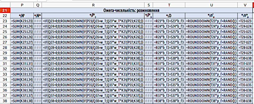

Fig. 4.9. Formulas in the second part of the "Three-Generation Model." Computations of male numbers are analogous to those of female numbers; the number of pairs with third-age females is computed analogously to the number of pairs with second-age females.
Columns P and Q compute the total number of sexually mature females and males, ωtNF and ωtNM respectively. The formulas are quite simple: P23{=SUM(K23:L23)}; the formula in cell Q23 is analogous. Clearly, these cells sum the numbers of sexually mature females and males of different ages.
Columns R and S compute the number of pairs with second-age and third-age females, ωtPf2 and ωtPf3 respectively. One must account for the possibility that males may be insufficient for all females, and the computation must therefore be: R23{=IF(Q23=0;0;ROUNDDOWN(IF(P23/Q23>w_T;Q23*w_T*K23/P23;K23);))}. The first IF function guards against division by zero, since it is subsequently necessary to divide the number of females by the number of males. If there are no males in the population, there are no pairs either. If males are present, it must be determined whether their number is sufficient to mate with all females. If the ratio of female to male numbers is less than ωT, the number of pairs with second-age females equals the number of second-age females, and the number of pairs with third-age females equals the number of third-age females. If males are deficient (it should be noted that under the conditions stipulated in the model this can occur only at the very first step, if an excess of females and a deficit of males is specified), then the number of pairs with females of both age groups is reduced proportionally to the available number of males: number_of_males * T * number_of_females_of_corresponding_age / number_of_females, or for second-age females in the first cycle Q23*w_T*K23/P23.
Column T computes the number of offspring (this quantity is denoted ωO, from the English "offspring"). For this purpose, the product of the number of pairs with second-age females and the fecundity of second-age females must be added to the product of the number of pairs with third-age females and the fecundity of third-age females: T23{=R23*b_f2+S23*b_f3}.
Column U contains the computation of the number of females appearing in the offspring. To compute this, one must account for their expected proportion in the offspring pf, which is among the initial parameters, and apply probabilistic rounding: U23{=ROUNDDOWN(T23*p_f+RAND();)}. The number of males in the offspring is determined very simply: V23{=T23-U23}. All computations of the cycle are complete; it remains to "stretch" the necessary formulas and to construct a graph from the data contained in columns P and Q.
4.3. Behavior of the Resulting Model
It is now worthwhile to reflect on certain aspects of the resulting model. As can be seen from its screenshot (Fig. 4.1), at certain combinations of input values the model exhibits oscillations that sometimes have the appearance of "beats." It is important to understand what causes them. What combinations of input coefficients produce these "beats"? How do situations at their minima and maxima differ from one another? Why, during the first few years under the input values shown in the figure, did the model population grow slowly, and then make a sudden "surge"?
Can one compute the ratio whose change causes "beats" in abundance? Can one construct a graph of such a quantity? Can one superimpose a graph of such a quantity on the graph of population dynamics?
Verify whether the oscillations in the model population abundance are related to a non-equilibrium sex ratio. If the oscillations are associated with other causes, one may set the input parameter pf to 0.5 and leave it unchanged during the analysis of model behavior.
Which of the simplifications adopted in constructing this model were the most significant? Probably the most serious simplification (closely related to the cause of the beats) is that mortality upon exceeding carrying capacity was the same for all age classes. The second serious simplification is that population abundance grows without any deceleration until it reaches carrying capacity, and is then abruptly trimmed to that level year after year.
In light of the foregoing, the direction of further model refinement and approximation to reality becomes clear. It is necessary to introduce separate mortality rates (and possibly competitiveness values) for different age classes (and probably for different sexes). The mechanism of competitive abundance reduction must be made more complex.
The program of further actions is beginning to take shape... Before all else, however, the posed question must be answered: with what processes are the periodic abundance oscillations in our three-generation model associated?
First of all, one may verify that these oscillations become more pronounced the greater the difference in fecundity between second-age and third-age individuals. This can be established simply by observing how changes in the initial parameters are reflected in the output graph. With equal fecundity of the two age groups, population abundance rapidly stabilizes at a given level.
What are the oscillations in abundance associated with? With the periodic change in the ratio between generations. Let us examine in detail how to visualize these changes, the more so as this will provide an opportunity to discuss the most elementary means of editing graphs.
We begin by increasing carrying capacity. The consequence will be that the oscillations begin to dampen. Using the model, one may experimentally verify that oscillations that have begun to dampen can intensify only in the case of a small carrying capacity. From this one may understand that the cause of oscillation intensification is the deviation in the generation ratio associated with the rounding procedure. The smaller the abundance of the model population, the greater the influence that random processes during probabilistic rounding can have on its dynamics.
Let us enter into one of the cells to the side of the computation zone the formula visible in Fig. 4.10. Above it we will make a label explaining what we are computing. For three columns demonstrating the dynamics of generations, we will construct a graph, placing it directly above the computation zone.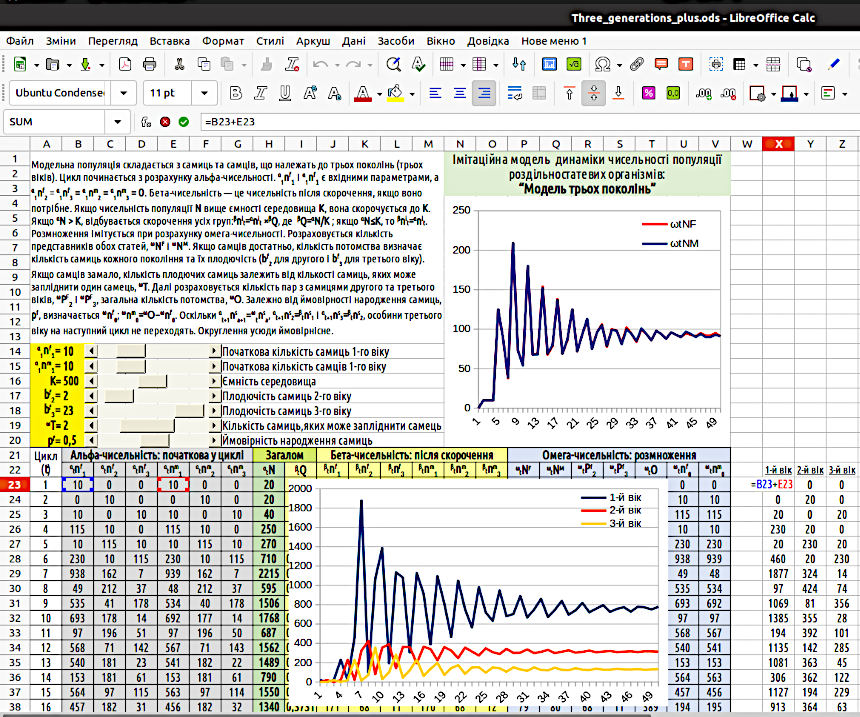

Fig. 4.10. Oscillations in the model population abundance are a consequence of oscillations in the inter-generational ratio.
The cause of the "beats" is oscillations in the ratio between generations! When the more numerous generation reaches the third age, this leads to a surge in offspring numbers, a sharp reduction in the numbers of individuals of all ages, and the formation of a less numerous generation. When that generation begins to reproduce, a larger number of offspring can remain in the model population, thus forming a more numerous generation... The aforementioned cyclical oscillations in the inter-generational ratio produce the cyclical "beats" in population abundance, which dampen over time. Eventually, abundance stabilizes, but any perturbation (for example, a substantial change in population size resulting from some external impact) will again produce "beats" in abundance, which will dampen over time under stable conditions.
An interesting way of presenting the same results is shown in Fig. 4.11, in the graph at the upper right. The data from the column describing the proportion of young individuals (as a percentage of total abundance) are plotted on the x-axis, while data on the proportion of third-year individuals are plotted on the y-axis. The broken curve traces the trajectory of the system in the phase space shown. The very first point is in the lower right corner of the given graph (100% young individuals). The next is at the origin of coordinates (all individuals are second-year). In the third year the generational ratio is approximately 50%/50% (individuals of the first generation have left offspring, and for each mating pair there are, according to the parameters shown in Fig. 4.11, two offspring). Construct such a graph yourself!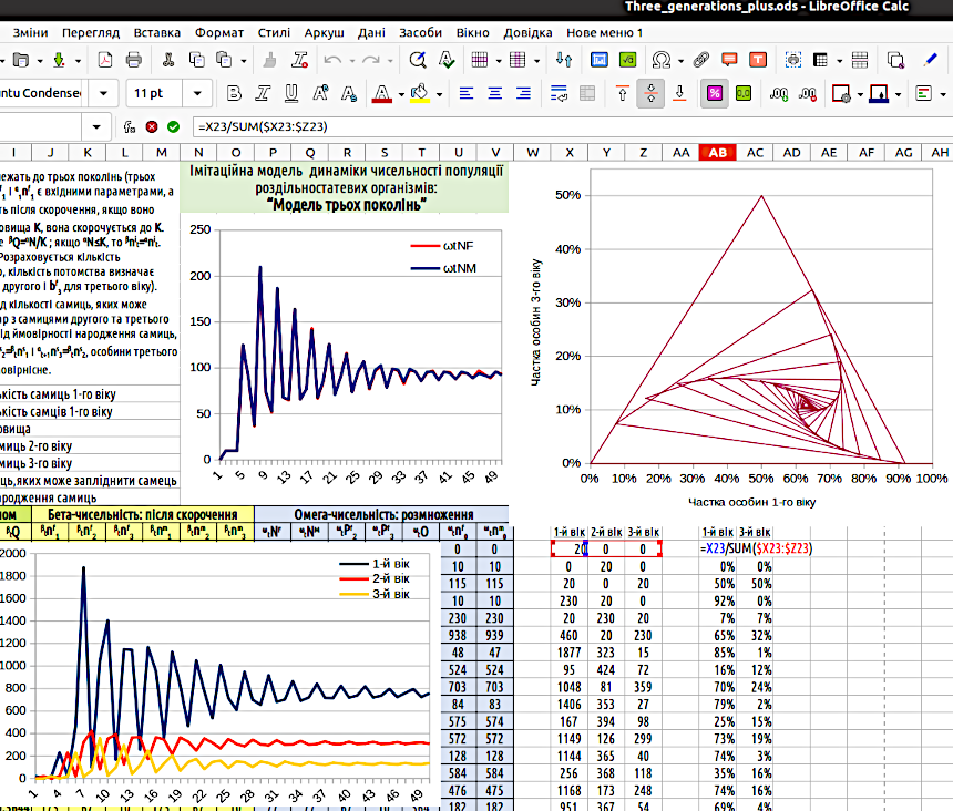

Fig. 4.11. Added is a graph demonstrating the trajectory of the model population in phase space. At each step the model system moves from one vertex of the broken line to the next. The starting point is in the lower right corner.
How realistic is the assumption that individuals of different ages equally deplete environmental resources and have equal survival probabilities in the event of competitive abundance reduction? This is most likely a very crude approximation. Experience of disasters associated with resource scarcity — both in human populations and in populations of other species — indicates that certain segments of the population prove to be especially vulnerable. The sex ratio and age-class composition of a population that has passed through a "starvation" reduction in numbers must shift substantially compared to the original composition.
4.4. The Logic of Simulation Model Construction
Building upon the model shown in Fig. 4.1, we may discuss yet another pedagogical problem. How is a model constructed? First, the model author divides the process under study into certain steps. Most models in this course operate by repeatedly cycling through a given cycle (for example, one corresponding to a year or a given generation). The events occurring at each cycle can be subdivided into certain stages. For example, the stages considered by our model are: computation of α-abundance at each cycle, determination of β-abundance (with reduction in case carrying capacity is exceeded), pair formation, and ω-abundance — the number of offspring. What, for example, influences α-abundance and determines its value? For the first (which we designate the zeroth) model cycle — the initial abundance, which is specified among the initial parameters. For all subsequent cycles, α-abundance depends on ω-abundance and the result of reproduction at the preceding stage. The set of such relationships is schematically depicted in Fig. 4.12.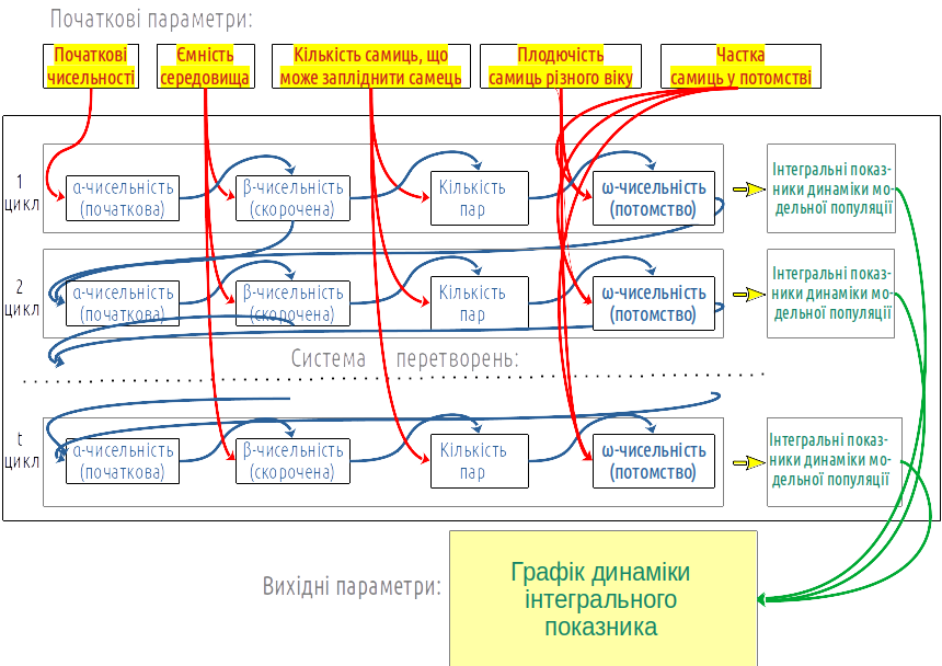

Fig. 4.12. Dependencies of the variables in the model are shown in this diagram by arrows. If we specify the formulas that determine these dependencies, we obtain a conceptual model. It can be implemented on a variety of software platforms.
For the computations that enter into the system of transformations, initial parameters must be defined. The result of the computations will be a certain output, for example, the dynamics of a given indicator. The integral indicator whose dynamics are displayed in the graph in Fig. 4.1 is the abundance of sexually mature females and males.
If we determine by what formulas all intermediate and final values are computed, we create a conceptual model. This model can be implemented on a variety of platforms (it could even be implemented on a set of slips of paper on which computed values are recorded, or, conversely, on one large sheet of paper). Naturally, it is better to do this on a computer using appropriate software. As you will understand, in this course we use LO Calc.
How did we do this? We allocated on the LO Calc worksheet a zone for input parameters, a calculation zone, and a results display zone. In the calculation zone, step by step, we wrote out the first (zeroth, in our numbering) cycle. From the results of this cycle we began the next. It is logical to place cycles in rows, and the various indicators computed at each cycle — in columns. The zeroth row can be "stretched" to the first; the difference between them concerns only how α-abundance is computed. The first row can then be "stretched" to all subsequent ones.
The means of displaying output results may take what Fig. 4.12 calls "integral indicators" either from the computations themselves or from a dedicated, separate block (as done, for example, in Fig. 4.10). If necessary, in addition to dynamics one may display a required indicator that permits comparing different model runs (for example, population abundance at the end of the 100th cycle).
Do you not feel a sense of wonder? We have placed a certain number of cells on a spreadsheet and linked them with straightforward formulas. Routine work — yet as a result of performing it, the model has "come to life." One can vary the initial parameters and observe how the behavior of the model changes. In certain cases these changes will be predictable, intuitively comprehensible; in others, on the contrary, counterintuitive. In any case, performing this work brings us one step closer to understanding the behavior of the original systems, to understanding reality — which no model can fully reflect.